Knowledge Repository
Xinyu Chen (陈新宇) created this page since early 2024 at MIT with the purpose of fostering research knowledge, vision, insight, and style from an interdisciplinary perspective. In the meantime, the knowledge repository aims to connect random concepts with mathematics and machine learning.
86th Commit
Conjugate Gradient Method
References:
[1] An Introduction to the Conjugate Gradient Method without the Agonizing Pain.
[2] Conjugate Direction Methods.
[3] Conjugate Gradient Descent.
[4] Numerical Analysis – Lecture 19.
85th Commit
Covariance Matrix & Eigenvalue Decomposition
Recently, we released an YouTube video about covariance matrix, answering why does eigenvalue decomposition define the shape of multivariate Gaussian, please check out YouTube for details. This video explains the geometric relationship between the eigenvalue decomposition of a covariance matrix and the shape of a multivariate Gaussian distribution.
- Multivariate Gaussian Overview: The distribution’s shape and center are defined by a mean vector and a covariance matrix.
- Geometric Interpretation: When visualizing a bivariate Gaussian, the level sets (points of equal probability density) form ellipsoids.
- Empirical Verification: The video demonstrates this geometry by generating random samples, showing how the data clusters align perfectly with the predicted elliptical shape as the sample size increases.
- Correlation Effects: By comparing positive and negative off-diagonal entries in the covariance matrix, the video illustrates how correlation effectively rotates the ellipse.
References:
[1] Why is the eigenvector of a covariance matrix equal to a principal component?
[2] A geometric interpretation of the covariance matrix.
[3] Covariance and Principal Components.
[4] Eigenvalues of covariance matrices.
[5] what does eigenvalues expres in the covariance matrix?
84th Commit
Huber’s Location Estimator
[1] Stanislav Nagy (2025). Robust Statistical Methods. Course note.
[2] Peter Rousseeuw (2019). Robust Statistics Part 1: Introduction and univariate data. Slides.
For the location model with the standard normal distribution $\Phi(x)$, we have \(-f_0'(x)/f_{0}(x)=x\) and
\[\tilde{\psi}(x)=[x-a]_{-b}^{b}\]Because of the symmetry of $\Phi$, for each $b>0$, we get
\[\int_{\mathbb{R}}[x]_{-b}^{b}d\Phi(x)=0\]which gives $a=0$. The Hampel optimal estimator at the normal location model is given by
\[\psi(x)=[x]_{-b}^{b}=\begin{cases} x, & \text{if $|x|<b$}, \\ \operatorname{sgn}(x)\cdot b, & \text{otherwise} \end{cases}\]This is the Huber’s M-estimator of location. The Huber estimator does not take an explicit form; for a random sample $X_1,\ldots,X_n$, it is computed as the solution in $t\in\mathbb{R}$ to
\[\sum_{i=1}^{n}\psi(X_i-t)=0\]or equivalently as $t\in\mathbb{R}$ that minimizes the Huber loss $\sum_{i=1}^{n}\rho(X_i-t)$ where
\[\rho(x)=\begin{cases} x^2/2, & \text{if $|x|<b$}, \\ b(|x|-b/2), & \text{otherwise} \end{cases}\]As $b\to\infty$, we get the squared loss function, and the estimator is just the sample average. As $b\to 0$, we approach the absolute loss and get the sample median.
83rd Commit
Random Matrix Theory for Portfolio Optimization
[1] Random Matrix Theory: Why does Wall Street use quantum physics? YouTube.
[2] Marchenko-Pastur law with relaxed independence conditions. arXiv.
The Markowitz theory has a curse of dimensions because of \(N(N-1)/2\) correlations for \(N\) portfolios. For example, 500 portfolios has 124,750 correlations, involving overwhelming noise.
In physics, Wigner’s leap claims the difficulty to compute exact interations and resolves it by a purely random matrix. The Marchenko-Pastur law describes what happens to the eigenvalues of purely noise.
Assume that \(\boldsymbol{Y}\) is a $p\times n$ random matrix whose entries are independent, identically distributed with a probability distribution $G$ on $\mathbb{R}$ with mean 0 and variance 1, and define a random matrix
\[\boldsymbol{S}=\frac{1}{n}\boldsymbol{Y}\boldsymbol{Y}^\top\]If and only if $p,n\to\infty$ in a way that $p/n\to y\in(0,1]$, then the empirical spectral distribution converges weakly to the Marchenko-Pastur distribution the density:
\[f_{y}(x)=\frac{\sqrt{(b-x)(x-a)}}{2\pi xy}\mathbf{1}_{[a,b]}(x)\]where $a$ and $b$ are functions of $y$, given by
\[a=a_y=(1-\sqrt{y})^2\quad\quad b=b_y=(1+\sqrt{y})^2\]82nd Commit
Sparse Quantile Regression
Source: Lan Wang,Yichao Wu, Runze Li (2012). Quantile Regression for Analyzing Heterogeneity in Ultra-High Dimension. Journal of the American Statistical Association. 107(497): 214–222.
Main Claims
I. Loss functions with sparsity.
SCAD penalty function:
\[\begin{aligned} p_{\lambda,a}(x)=&\lambda|x|\mathbb{I}\{0\leq|x|<\lambda\} \\ &+\frac{a\lambda|x|-(x^2+\lambda^2)/2}{a-1}\mathbb{I}\{\lambda\leq|x|\leq a\lambda\} \\ &+\frac{(a+1)\lambda^2}{2}\mathbb{I}\{|x|>a\lambda\} \end{aligned} \tag{82-1}\]for any $a>2$.
MCP penalty function:
\[p_{\lambda,a}(\beta)=\lambda\Bigl(|\beta|-\frac{\beta^2}{2a\lambda}\Bigr)\mathbb{I}\{0\leq|\beta|<a\lambda\}+\frac{a\lambda^2}{2}\mathbb{I}\{|\beta|>a\lambda\} \tag{82-2}\]for any $a>1$.
For the function:
\[g(\boldsymbol{\beta})=\frac{1}{n}\sum_{i=1}^{n}\rho_{\tau}(y_i-\boldsymbol{x}_i^\top\boldsymbol{\beta})+\lambda\sum_{j=1}^{p}|\beta_j| \tag{82-3}\]The subgradient of $g(\boldsymbol{\beta})$ is given by
\[\begin{aligned} \frac{\partial g(\boldsymbol{\beta})}{\partial\beta_{j}}=&-\frac{\tau}{n}\sum_{i=1}^{n}x_{ij}\mathbb{I}\{y_i-\boldsymbol{x}_i^\top\boldsymbol{\beta}>0\} \\ &+\frac{1-\tau}{n}\sum_{i=1}^{n}x_{ij}\mathbb{I}\{y_{i}-\boldsymbol{x}_i^\top\boldsymbol{\beta}<0\} \\ &-\frac{1}{n}\sum_{i=1}^{n}x_{ij}v_{i}+\lambda l_j \end{aligned} \tag{82-4}\]where
\[v_{i}=\begin{cases} 0, & \text{if}~y_i-\boldsymbol{x}_i^\top\boldsymbol{\beta}\neq0, \\ c\in[\tau-1,\tau], &\text{otherwise} \end{cases} \tag{82-5}\]II. Local linear approximation (LLA) algorithms.
The aforementioned optimization problem can be solved by using the LLA algorithm.
While minimizing
\[\min_{\boldsymbol{\beta}}~\frac{1}{n}\sum_{i=1}^{n}\rho_{\tau}(y_i-\boldsymbol{x}_i^\top\boldsymbol{\beta})+\sum_{j=1}^{p}p_{\lambda,a}(|\beta_j|) \tag{82-6}\]we initialize by setting $\tilde{\beta}_j^{(0)},\,\forall j$. For each step $t\geq1$, we update by solving
\[\min_{\boldsymbol{\beta}}~\frac{1}{n}\sum_{i=1}^{n}\rho_{\tau}(y_i-\boldsymbol{x}_i^\top\boldsymbol{\beta})+\sum_{j=1}^{p}w_{j}^{(t-1)}|\beta_j| \tag{82-7}\]which can be reformulated as a linear programming problem:
\[\begin{aligned} \min_{\boldsymbol{\xi}^{+}\geq0,\,\boldsymbol{\xi}^{-}\geq0,\,\boldsymbol{\zeta}}~&\frac{1}{n}\sum_{i=1}^{n}\left(\tau\xi_{i}^{+}+(1-\tau)\xi_{i}^{-}\right)+\sum_{j=1}^{p}w_{j}^{(t-1)}\zeta_{j} \\ \text{s.t.}~&y_{i}-\boldsymbol{x}_i^\top\boldsymbol{\beta}-\xi_{i}^{+}+\xi_{i}^{-}=0,&\forall i \\ &\zeta_j\geq\beta_j,\,\zeta_j\geq-\beta_j,&\forall j \end{aligned} \tag{82-8}\]The weights are updated by the subgradients:
\[w_j^{(t-1)}=\frac{\partial p_{\lambda,a}(|\tilde{\beta}_{j}^{(t-1)}|)}{\partial\tilde{\beta}_{j}^{(t-1)}}\geq0,\quad\text{consider}~w_j^{(0)}=\lambda \tag{82-9}\]If the weights $w_j^{(t)}$ stable, i.e., \(\displaystyle\sum_{j=1}^{p}(w_{j}^{(t-1)}-w_{j}^{(t)})^2\) is sufficiently small, then it could claim convergence of the LLA algorithm.
81st Commit
Nonparametric Quantile Estimation
Source: Takeuchi, I., Le, Q., Sears, T., & Smola, A. (2006). Nonparametric quantile estimation. Journal of Machine Learning Research. 7(45): 1231–1264.
Main Claims
I. Show the relation to support vector regression.
The loss of quantile regression with the $\tau$-th conditional quantile, i.e., $\tau\in(0,1)$, is
\[\ell_{\tau}({\varepsilon})=\begin{cases} \tau{\varepsilon}, & \text{if}~{\varepsilon}\geq{0}, \\ (1-\tau){\varepsilon}, & \text{otherwise} \tag{81-1} \end{cases}\]For any function $y=\langle\phi(\boldsymbol{x}),\boldsymbol{w}\rangle+b$, the optimization is given by
\[\begin{aligned} \min_{\boldsymbol{w},\,b,\,{\varepsilon}_i,\,{\varepsilon}_i^{*}}\quad &\frac{1}{\lambda m}\sum_{i=1}^{m}\left(\tau{\varepsilon}_i+(1-\tau){\varepsilon}_i^{*}\right)+\frac{1}{2}\|\boldsymbol{w}\|_2^2 \\ \text{s.t.}\quad &\color{blue}-{\varepsilon}_i^{*}\leq y_i-\langle\phi(\boldsymbol{x}_i),\boldsymbol{w}\rangle-b\leq{\varepsilon}_i,\quad{\varepsilon}_i,{\varepsilon}_i^{*}\geq0,\quad\forall i \end{aligned} \tag{81-2}\]where the dual constraints for $\boldsymbol{\varepsilon}$ and $\boldsymbol{\varepsilon}^{*}$ can be combined into one variable. This yields the following dual optimization:
\[\begin{aligned} \min_{\boldsymbol{\alpha}}\quad &\frac{1}{2}\boldsymbol{\alpha}^\top\boldsymbol{K}\boldsymbol{\alpha}-\boldsymbol{\alpha}^\top\boldsymbol{y} \\ \text{s.t.}\quad &\frac{\tau-1}{\lambda m}\leq\alpha_i\leq\frac{\tau}{\lambda m},\quad\mathbb{I}_{m}^\top\boldsymbol{\alpha}=0 \end{aligned} \tag{81-3}\]Then we use the kernel expression:
\[\boldsymbol{w}=\sum_{i=1}^{m}\alpha_i\phi(\boldsymbol{x}_i)\quad\Rightarrow\quad y=\sum_{i=1}^{m}\alpha_i\cdot k(\boldsymbol{x}_i,\boldsymbol{x})+b \tag{81-4}\]II. Linear programming regularization.
\[\min_{\alpha_i}~\frac{1}{m}\sum_{i=1}^{m}\ell_{\tau}\Bigl(y_i-\sum_{j=1}^{n}\left(\alpha_jf_{j}(\boldsymbol{x}_i)+b\right)\Bigr)+\lambda\sum_{j=1}^{n}|\alpha_j| \tag{81-5}\]III. Monotonicity and non-crossing quantiles.
Suppose that we want to estimate $n$ conditional quantiles at $0<\tau_1<\tau_2<\cdots<\tau_n<1$. The primal optimization problem is given by
\[\begin{aligned} \min_{\boldsymbol{w}_h,\,b_h,\,{\varepsilon}_{hi},\,{\varepsilon}_{hi}^{*}}\quad &\sum_{h=1}^{n}\Bigl(\frac{1}{\lambda m}\sum_{i=1}^{m}\left(\tau_h{\varepsilon}_{hi}+(1-\tau_h){\varepsilon}_{hi}^{*}\right)+\frac{1}{2}\|\boldsymbol{w}_h\|_2^2\Bigr) \\ \text{s.t.}\quad &\color{blue}y_{i}-\langle\phi(\boldsymbol{x}_i),\boldsymbol{w}_{h}\rangle-b_h-{\varepsilon}_{hi}+{\varepsilon}_{hi}^{*}=0,\quad{\varepsilon}_{hi},{\varepsilon}_{hi}^{*}\geq0,&\forall h,i \\ &\underbrace{\color{red}\langle\phi(\boldsymbol{x}_i),\boldsymbol{w}_{h+1}\rangle+b_{h+1}\geq\langle\phi(\boldsymbol{x}_i),\boldsymbol{w}_h\rangle+b_h}_{\text{non-crossing constraints}},&\forall h,i \end{aligned} \tag{81-6}\]80th Commit
$\ell_1$- and $\ell_{\infty}$-Norm of Matrices
Source: Matrix norms.
For any matrix \(\boldsymbol{A}\in\mathbb{R}^{m\times n}\), the $\ell_1$-norm is defined as:
\[\|\boldsymbol{A}\|_{1}=\max_{1\leq j\leq n}\,\sum_{i=1}^{m}|a_i|\]While the $\ell_{\infty}$-norm is defined as:
\[\|\boldsymbol{A}\|_{\infty}=\max_{1\leq i\leq m}\,\sum_{j=1}^{n}|a_j|\]79th Commit
Linear Programming Examples
Source: Introduction to convex optimization.
In linear programming, both objective function and constraints are linear:
\[\begin{aligned} \min_{\boldsymbol{x}}\quad&\boldsymbol{c}^\top\boldsymbol{x} \\ \text{s.t.}\quad&\boldsymbol{A}\boldsymbol{x}\leq\boldsymbol{b} \\ &\boldsymbol{x}\geq0 \end{aligned} \tag{79-1}\]where the vectors \(\boldsymbol{c},\boldsymbol{b}\) and the matrix \(\boldsymbol{A}\) are the parameters specifying the objective function and constraints.
Example 1. (\(\ell_1\)-norm regression as linear programming) Minimizing any vector norm of linear regression \(\boldsymbol{A}\boldsymbol{x}-\boldsymbol{b}\) is a convex optimization. We can reformulate minimizing \(\|\boldsymbol{A}\boldsymbol{x}-\boldsymbol{b}\|_1\) over \(\boldsymbol{x}\) as a linear programming:
\[\begin{aligned} \min_{\boldsymbol{x},\,\boldsymbol{t}}\quad&\sum_{i}t_i \\ \text{s.t.}\quad&-t_i\leq[\boldsymbol{A}\boldsymbol{x}-\boldsymbol{b}]_i\leq t_i &\forall i \\ &t_i\geq 0 &\forall i \end{aligned} \tag{79-2}\]with \(t_1,t_2,\ldots,t_n\) as auxiliary decision variables.
Example 2. (\(\ell_{\infty}\)-norm regression as linear programming) Infinity norm for a vector is defined by the “worst-case” maximum absolute value. We can reformulate the regression problem as a linear programming:
\[\begin{aligned} \min_{\boldsymbol{x},\,t}\quad& t \\ \text{s.t.}\quad&-t\leq[\boldsymbol{A}\boldsymbol{x}-\boldsymbol{b}]_i\leq t&\forall i \\ &t\geq0 \end{aligned} \tag{79-3}\]with $t$ as a single auxiliary decision variable.
78th Commit
GPU-Accelerated Mixed Integer Programming
Source: Akif Çördük, Piotr Sielski, Alice Boucher, Kumar Aatish (2025). GPU-Accelerated Primal Heuristics for Mixed Integer Programming. arXiv:2510.20499. [Blog post]
NVIDIA cuOpt leverages GPU acceleration to implement advanced primal heuristics, such as a GPU-optimized feasibility pump (FP) with first-order PDLP solvers and domain propagation, achieving significant speedups and improved solution quality for large-scale MIP instances, including previously unsolved MIPLIB benchmarks.
77th Commit
Second-Order Cone Programming
Source: Second-order cone program.
Given the data \(\boldsymbol{f}\in\mathbb{R}^{n}\), \(\boldsymbol{F}\in\mathbb{R}^{p\times n}\), and \(\boldsymbol{g}\in\mathbb{R}^{p}\), in the meantime suppose \(\boldsymbol{A}_{i}\in\mathbb{R}^{n_i\times n}\), \(\boldsymbol{b}_{i}\in\mathbb{R}^{n_i}\), \(\boldsymbol{c}_{i}\in\mathbb{R}^{n}\), and \(d_{i}\) for all \(i\in\{1,2,\ldots,m\}\), a second-order cone program (SOCP) is an optimization problem of the form
\[\begin{aligned} \min_{\boldsymbol{x}}\quad&\boldsymbol{f}^{\top}\boldsymbol{x} \\ \text{s.t.}\quad&\|\boldsymbol{A}_{i}\boldsymbol{x}+\boldsymbol{b}_{i}\|_2\leq\boldsymbol{c}_{i}^\top\boldsymbol{x}+d_i,\quad\forall i \\ &\boldsymbol{F}\boldsymbol{x}=\boldsymbol{g} \end{aligned} \tag{77-1}\]An example of an SOCP is the robust linear programming such that
\[\begin{aligned} \min_{\boldsymbol{x}}\quad&\boldsymbol{c}^\top\boldsymbol{x} \\ \text{s.t.}\quad&\boldsymbol{a}_{i}^\top\boldsymbol{x}+\|\boldsymbol{x}\|_2\leq b_i,\quad\forall i \end{aligned} \tag{77-2}\]76th Commit
Sequential Quadratic Programming
Reference: Alex Oshin, Rahul Vodeb Ghosh, Augustinos D. Saravanos, Evangelos A. Theodorou (2025). Deep FlexQP: Accelerated Nonlinear Programming via Deep Unfolding. arXiv:2512.01565.
Nonlinear programming is a challenging problem in large-scale decision-making processes. Sequential quadratic programming (SQP) methods utilizes quadratic programming to solve complicated problems in which the objective and constraints may be nonlinear and nonconvex. For the nonlinear programming such that
\[\begin{aligned} \min_{\boldsymbol{x}\in\mathbb{R}^{n}}\quad&\underbrace{f(\boldsymbol{x})}_{\color{red}\text{twice-differentiable}} \\ \text{s.t.}\quad&\underbrace{g(\boldsymbol{x})\leq0}_{\color{red}\text{inequality}} \quad \underbrace{h(\boldsymbol{x})=0}_{\color{red}\text{equality}} \\ \end{aligned} \tag{76-1}\]with $g:\mathbb{R}^{n}\to\mathbb{R}^{m}$ and $h:\mathbb{R}^{n}\to\mathbb{R}^{p}$ describe the inequality and equality constraints, respectively. Indeed, SQP solves this nonlinear programming problem by linearizing the constraints and quadraticizing the Lagrangian
\[\mathcal{L}(\boldsymbol{x},\boldsymbol{y}_{I},\boldsymbol{y}_{E})=f(\boldsymbol{x})+\boldsymbol{y}_{I}^\top g(\boldsymbol{x})+\boldsymbol{y}_{E}^\top h(\boldsymbol{x}) \tag{76-2}\]around the current iterate \((\boldsymbol{x}^{k},\boldsymbol{y}_{I}^{k},\boldsymbol{y}_{E}^{k})\) with dual variables \(\boldsymbol{y}_{I}\in\mathbb{R}_{+}^{m}\) and \(\boldsymbol{y}_{E}\in\mathbb{R}^{p}\). Let the Henssian matrix be
\[H_{\boldsymbol{x}}\triangleq\nabla_{\boldsymbol{x}}\mathcal{L}(\boldsymbol{x},\boldsymbol{y}_{I},\boldsymbol{y}_{E})\]Eq. (76-1) can be thus converted into the following quadratic programming subproblem:
\[\begin{aligned} \min_{\boldsymbol{w}}\quad&\frac{1}{2}\boldsymbol{w}^\top H_{\boldsymbol{x}^{k}}\boldsymbol{w}+\nabla f(\boldsymbol{x}^{k})^\top\boldsymbol{w} \\ \text{s.t.}\quad&g(\boldsymbol{x}^{k})+\nabla g(\boldsymbol{x}^{k})^\top\boldsymbol{w}\leq 0 \\ &h(\boldsymbol{x}^{k})+\nabla h(\boldsymbol{x}^{k})^\top\boldsymbol{w}=0 \end{aligned} \tag{76-3}\]75th Commit
A Convex Binary Reformulation of Sparse Linear Regression
Reference: Dimitris Bertsimas, Bart Van Parys (2020). Sparse high-dimensional regression: Exact scalable algorithms and phase transitions. The Annuals of Statistics. 48 (1): 300-323.
Given design matrix $\boldsymbol{X}\in\mathbb{R}^{n\times p}$ and response vector $\boldsymbol{y}\in\mathbb{R}^{n}$, the problem of linear regression with $\ell_0$-norm sparsity constraint is defined as follows,
\[\begin{aligned} \min_{\boldsymbol{w}}\quad&\frac{1}{2}\|\boldsymbol{y}-\boldsymbol{X}\boldsymbol{w}\|_2^2+\frac{1}{2\lambda}\|\boldsymbol{w}\|_2^2 \\ \text{s.t.}\quad&\|\boldsymbol{w}\|_0\leq k \end{aligned}\tag{75-1}\]where $\lambda>0$ is a weight that controls the importance of the regularization term.
Let $\Omega=\operatorname{supp}(\boldsymbol{w})$ be the support set and $q=\operatorname{card}(\Omega)$, the closed-form solution to the optimization problem is given by
\[\boldsymbol{w}_{\Omega}:=(\boldsymbol{X}_{\Omega}^\top\boldsymbol{X}_{\Omega}+\boldsymbol{I}_{q}/\lambda)^{-1}\boldsymbol{X}_{\Omega}^\top\boldsymbol{y} \tag{75-2}\]Thus, the objective function can be written as follows,
\[\begin{aligned} f=&\frac{1}{2}\boldsymbol{y}^\top\boldsymbol{y}-{\color{red}\boldsymbol{w}_{\Omega}^\top\boldsymbol{X}_{\Omega}^\top\boldsymbol{y}}+{\color{blue}\frac{1}{2}\boldsymbol{w}_{\Omega}^\top(\boldsymbol{X}_{\Omega}^\top\boldsymbol{X}_{\Omega}+\boldsymbol{I}_{q}/\lambda)\boldsymbol{w}_{\Omega}} \\ =&\frac{1}{2}\boldsymbol{y}^\top\boldsymbol{y}-{\color{red}\boldsymbol{y}^\top\boldsymbol{X}_{\Omega}(\boldsymbol{X}_{\Omega}^\top\boldsymbol{X}_{\Omega}+\boldsymbol{I}_q/\lambda)^{-1}\boldsymbol{X}_{\Omega}^\top\boldsymbol{y}} \\ &\quad+{\color{blue}\frac{1}{2}\boldsymbol{y}^\top\boldsymbol{X}_{\Omega}(\boldsymbol{X}_{\Omega}^\top\boldsymbol{X}_{\Omega}+\boldsymbol{I}_{q}/\lambda)^{-1}\boldsymbol{X}_{\Omega}^\top\boldsymbol{y}} \\ =&\frac{1}{2}\boldsymbol{y}^\top\boldsymbol{y}-\frac{1}{2}\boldsymbol{y}^\top\boldsymbol{X}_{\Omega}(\boldsymbol{X}_{\Omega}^\top\boldsymbol{X}_{\Omega}+\boldsymbol{I}_q/\lambda)^{-1}\boldsymbol{X}_{\Omega}^\top\boldsymbol{y} \\ =&\frac{1}{2}\boldsymbol{y}^\top{\color{orange}\left(\boldsymbol{I}_{n}-\boldsymbol{X}_{\Omega}(\boldsymbol{X}_{\Omega}^\top\boldsymbol{X}_{\Omega}+\boldsymbol{I}_q/\lambda)^{-1}\boldsymbol{X}_{\Omega}^\top\right)}\boldsymbol{y} \\ =&\frac{1}{2}\boldsymbol{y}^\top{\color{orange}(\boldsymbol{I}_n+\lambda\boldsymbol{X}_{\Omega}\boldsymbol{X}_{\Omega}^\top)^{-1}}\boldsymbol{y} \end{aligned} \tag{75-3}\]where the last line uses the matrix inverse lemma found by William W. Hager in 1989:
\[(\boldsymbol{I}_n+\lambda\boldsymbol{X}\boldsymbol{X}^\top)^{-1}=\boldsymbol{I}_n-\boldsymbol{X}(\boldsymbol{X}^\top\boldsymbol{X}+\boldsymbol{I}_{p}/\lambda)^{-1}\boldsymbol{X}^\top \tag{75-4}\]Then, the optimization problem of sparse regression can be reformulated a convex integer optimization:
\[\begin{aligned} \min_{\Omega}\quad&\frac{1}{2}\boldsymbol{y}^\top(\boldsymbol{I}_n+\lambda\boldsymbol{X}_{\Omega}\boldsymbol{X}_{\Omega}^\top)^{-1}\boldsymbol{y} \\ \text{s.t.}\quad&\operatorname{card}(\Omega)\leq k \end{aligned} \tag{75-5}\]74th Commit
Quadratic Programming over Huber Loss Function
Reference: Optimization Examples - Quadratic Programming.
For the Huber loss function such that
\[\phi(u)=\begin{cases} u^2 & \text{if $|u|<\delta$} \\ \delta(2|u|-\delta) &\text{otherwise} \end{cases} \tag{74-1}\]with any positive Huber threshold $\delta>0$, minimizing the Huber loss function is equivalent to the following quadratic programming problem (Exercise 6.3(c) in Convex Optimization, see page 344):
\[\begin{aligned} \min_{\alpha,\gamma}\quad&\gamma^2+2\delta\alpha \\ \text{s.t.}\quad&-\alpha\leq u-\gamma\leq\alpha,\quad\alpha\geq 0 \end{aligned} \tag{74-2}\]where $\alpha$ and $\gamma$ are continuous decision variables.
73rd Commit
Portfolio Selection (Definition)
Reference: Dimitris Bertsimas, Ryan Cory-Wright (2022). A Scalable Algorithm for Sparse Portfolio Selection. INFORMS Journal on Computing. 34 (3): 1489–1511.
For a universe of $n$ securities, we estimate a mean $\boldsymbol{\mu}\in\mathbb{R}^{n}$ (or return) and a covariance matrix $\boldsymbol{\Sigma}\in\mathbb{R}^{n\times n}$. The Markowitz model proposed in 1952 selects a portfolio that provides the highest expected return for a given amount of variance. The mean-variance portfolio optimization laid the foundation of modern portfolio theory, which can be formulated as follows,
\[\begin{aligned} \min_{\boldsymbol{x}\in\mathbb{R}_{+}^{n}}\quad&\frac{\lambda}{2}\boldsymbol{x}^\top\boldsymbol{\Sigma}\boldsymbol{x}-\boldsymbol{\mu}^\top\boldsymbol{x} \\ \text{s.t.}\quad&\boldsymbol{e}^\top\boldsymbol{x}=1 \\ \end{aligned} \tag{73-1}\]where $\lambda$ is a parameter that controls the trade-off between the portfolio’s risk and return, and $\boldsymbol{e}\in\mathbb{R}^{n}$ denotes the vector of all ones. As the decision variables, $\boldsymbol{x}$ denotes the portfolio allocation vector.
72nd Commit
Local Linear Approximation for Nonconvex Penalties
Reference: Jianqing Fan, Jinchi Lv, Lei Qi (2011). Sparse high-dimensional models in economics. Annual Review of Economics. 3, 291-317. [PDF]
Nonconvex penalties such as SCAD and MCP for sparse modeling are more flexible than LASSO. Given the decision variables $\boldsymbol{w}\in\mathbb{R}^{d}$, the local linear approximation (LLA, see Zou, 2008) is
\[\rho_{\lambda}(|w_k|)\approx\rho_{\lambda}(|w_k^{*}|)+\rho_{\lambda}^{\prime}(|w_k^{*}|)(|w_k|-|w_k^{*}|)\quad\text{for $w_k\approx w_k^{*}$} \tag{72-1}\]which is a convex majorant of a concave penalty function $\rho_{\lambda}(\cdot)$ on $[0,\infty)$.
The penalized least-squares (PLS) estimation can therefore be formulated as follows,
\[\min_{\boldsymbol{w}}\quad\frac{1}{2n}\|\boldsymbol{y}-\boldsymbol{X}\boldsymbol{w}\|_2^2+\sum_{k=1}^{d}\underbrace{\alpha_k|w_k|}_{\approx\rho_{\lambda}(|w_k|)} \tag{72-2}\]where $\boldsymbol{X}\in\mathbb{R}^{n\times d}$ and $\boldsymbol{y}\in\mathbb{R}^{n}$ are design matrix and response vector, respectively. The weights are
\[\alpha_k=\rho_{\lambda}^{\prime}(|w_k^{*}|) \tag{72-3}\]In the case of SCAD, the derivative is given by
\[\rho_{\lambda}^{\prime}(w)=\lambda\left(I\{w\leq\lambda\}+\frac{(a\lambda-w)_{+}}{(a-1)\lambda}I\{w>\lambda\}\right) \tag{72-4}\]for some $a>2$. Here, $\rho_{\lambda}(0)=0$ and $a=3.7$ is often used.
In the case of MCP, the derivative is given by
\[\rho_{\lambda}^{\prime}(w)=\frac{(a\lambda-w)_{+}}{a} \tag{72-5}\]In fact, if the initial estimate is zero, then $\alpha_k=\lambda$, and the resulting estimate is the LASSO estimate. Nonconvex penalties further reduce the bias problem of LASSO by assigning an adapative weighting scheme.
71st Commit
Automatic Lag Selection with Support Vector Regression
Reference: Sebastián Maldonado, Agustín González, Sven Crone (2019). Automatic time series analysis for electric load forecasting via support vector regression. Applied Soft Computing. 83, 105616.
The $\epsilon$-SVR method aims to solve the following optimization problem:
\[\begin{aligned} \min_{\boldsymbol{w},b,\boldsymbol{\xi}\geq0,\boldsymbol{\xi}^{*}\geq0}\quad&\frac{1}{2}\|\boldsymbol{w}\|_2^2+\lambda\sum_{i=1}^{n}(\xi_i+\xi_i^{*}) \\ \text{s.t.}\quad&y_i-(\boldsymbol{w}^\top\boldsymbol{x}_{i}+b)-\epsilon\geq\xi_{i},\quad\forall i\in\{1,2,\ldots,n\} \\ &(\boldsymbol{w}^\top\boldsymbol{x}_{i}+b)-y_i-\epsilon\geq\xi_{i}^{*}, \quad\forall i\in\{1,2,\ldots,n\} \\ \end{aligned} \tag{71-1}\]taking from the $\epsilon$-insensitive loss function such that
\[L_{\epsilon}(y,f(x))=\max(0,|y-f(x)|-\epsilon) \tag{71-2}\]where loss is zero if the absolute error is within $\epsilon$.
70th Commit
High-Dimensional Quantile Tensor Regression
Reference: Wenqi Lu, Zhongyi Zhu, Heng Lian (2020). High-dimensional Quantile Tensor Regression. Journal of Machine Learning Research. 21: 1-31.
Modern machine learning applications involve tensor data in the form of quantile regression such that
\[Q_{\tau}(y\mid\boldsymbol{\mathcal{X}})=\langle\boldsymbol{\mathcal{A}},\boldsymbol{\mathcal{X}}\rangle \tag{70-1}\]for the $\tau$th conditional quantile of response given $\boldsymbol{\mathcal{X}}\in\mathbb{R}^{p_1\times p_2\times \cdots \times p_{K}}$ and $y\in\mathbb{R}$. In the regressor, $\boldsymbol{\mathcal{A}}$ can be parameterized by the Tucker decomposition:
\[\boldsymbol{\mathcal{A}}=\boldsymbol{\mathcal{G}}\times_1\boldsymbol{U}_1\times_2\boldsymbol{U}_2\cdots\times_{K}\boldsymbol{U}_{K} \tag{70-2}\]Considering the loss of quantile regression as follows,
\[\rho_{\tau}(u)=\begin{cases} \tau u & \text{if $u>0$} \\ (\tau-1)u & \text{otherwise} \end{cases} \tag{70-3}\]By integrating tensor decomposition into quantile regression, we have
\[\begin{aligned} \min_{\boldsymbol{\mathcal{G}},\boldsymbol{U}_{1},\boldsymbol{U}_2,\cdots,\boldsymbol{U}_{K}}\quad&\sum_{i=1}^{n}\rho_{\tau}(y_i-\langle\boldsymbol{\mathcal{G}}\times_1\boldsymbol{U}_1\times_2\boldsymbol{U}_2\cdots\times_{K}\boldsymbol{U}_{K},\boldsymbol{\mathcal{X}}_{i}\rangle) \\ &\quad +\lambda\|\boldsymbol{U}_K\otimes\cdots\otimes\boldsymbol{U}_1\|_1 \\ \text{s.t.}\quad &\boldsymbol{U}_k^\top\boldsymbol{U}_k=\boldsymbol{I},\quad\forall k\in\{1,2,\ldots,K\} \end{aligned} \tag{70-4}\]with an $\ell_1$-norm induced sparsity penalty and orthogonality constraints on factor matrices.
Estimating these factor matrices can be converted into the following optimization problem:
\[\begin{aligned} \min_{\boldsymbol{r},\boldsymbol{U}}\quad&\rho_{\tau}(\boldsymbol{r})+\lambda\|\boldsymbol{U}\|_1 \\ \text{s.t.}\quad&\boldsymbol{r}=\boldsymbol{y}-\boldsymbol{Z}\operatorname{vec}(\boldsymbol{U}),\quad\boldsymbol{U}^\top\boldsymbol{U}=\boldsymbol{I} \end{aligned} \tag{70-5}\]69th Commit
Non-Quadratic Losses
Reference: Sanjay Lall and Stephen Boyd. Non-Quadratic Losses. EE104 at Stanford University.
The Huber loss has linear growth for large residual $r$ that makes fit less sensitive to outliers. Thus, empirical risk minimization (ERM) with Huber loss is called a robust prediction method. The log Huber loss is
\[\phi(u)=\begin{cases} u^2 & \text{if $|u|<\delta$} \\ \delta^2(1-2\operatorname{log}(\delta)+\operatorname{log}(u^2)) &\text{otherwise} \end{cases} \tag{69-1}\]for any positive parameter $\delta>0$.
68th Commit
Regression & Statistical Estimation (CVXPY x NASA Course 2024)
Huber penalty function with the Huber threshold $\delta>0$ has linear growth for large $u$ that makes approximation less sensitive to outliers:
\[\phi(u)=\begin{cases} u^2 & \text{if $|u|<\delta$} \\ \delta(2|u|-\delta) &\text{otherwise} \end{cases} \tag{68-1}\]So, it is also called robust penalty.
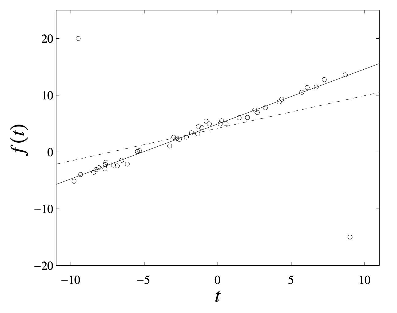
[Excellent example from page 300 of the convex optimization book] Affine function fitted on 42 points (with two outliers) using quadratic (dashed) and Huber (solid) penalty.
Given $\boldsymbol{A}\in\mathbb{R}^{m\times n}$ and $\boldsymbol{b}\in\mathbb{R}^{m}$ with $m$ measurements and $n$ regressors, when it minimizes residual $\boldsymbol{r}=\boldsymbol{A}\boldsymbol{x}-\boldsymbol{b}\in\mathbb{R}^{m}$, the optimization can be formulated to the following form:
\[\begin{aligned} \min_{\boldsymbol{x},\boldsymbol{r}}\quad&\sum_{i=1}^{m}\phi(r_i) \\ \text{s.t.}\quad&\boldsymbol{r}=\boldsymbol{A}\boldsymbol{x}-\boldsymbol{b} \\ \end{aligned} \tag{68-2}\]where $\phi:\mathbb{R}\to\mathbb{R}$ is a convex penalty function. In particular, Huber loss would lead to the robust regression.
As an alternative, quantile regression for any $\tau\in(0,1)$ takes the following form:
\[\begin{aligned} \min_{\boldsymbol{x},\boldsymbol{r}\geq0,\boldsymbol{r}^{*}\geq0}\quad&\sum_{i=1}^{m}\left(\tau r_{i}+(1-\tau) r_{i}^{*}\right) \\ \text{s.t.}\quad&\boldsymbol{r}-\boldsymbol{r}^{*}=\boldsymbol{A}\boldsymbol{x}-\boldsymbol{b} \\ \end{aligned} \tag{68-3}\]where $\boldsymbol{r}$ and $\boldsymbol{r}^{*}$ are over-estimated and under-estimated residual vectors, respectively.
- For $\tau=\frac{1}{2}$, same penalty for under-estimate and over-estimate.
- For $\tau>\frac{1}{2}$, higher penalty to under-estimate than over-estimate.
- For $\tau<\frac{1}{2}$, higher penalty to over-estimate than under-estimate.
67th Commit
Linear Algebra & Robot Control
Preliminaries
The column space $\mathcal{C}(\boldsymbol{A})$ of a matrix $\boldsymbol{A}$ is the span of its columns, i.e., the set of all linear combinations of the columns of $\boldsymbol{A}$:
\[\mathcal{C}(\boldsymbol{A})=\{\boldsymbol{A}\boldsymbol{x}\mid \boldsymbol{x}\in\mathbb{R}^{n}\} \tag{67-1}\]The nullspace $\mathcal{N}(\boldsymbol{A})$ of a matrix $\boldsymbol{A}$ is the set of all vectors $\boldsymbol{x}$ for which $\boldsymbol{A}\boldsymbol{x}=\boldsymbol{0}$ such that
\[\mathcal{N}(\boldsymbol{A})=\{\boldsymbol{x}\in\mathbb{R}^{n}\mid \boldsymbol{A}\boldsymbol{x}=\boldsymbol{0}\} \tag{67-2}\]The condition number of a square matrix $\boldsymbol{A}$ is defined as the ratio between the largest and smallest singular values, i.e.,
\[\kappa(\boldsymbol{A})=\frac{\sigma_{\text{max}}(\boldsymbol{A})}{\sigma_{\text{min}}(\boldsymbol{A})} \tag{67-3}\]measuring how much the solution $\boldsymbol{x}$ of $\boldsymbol{A}\boldsymbol{x}=\boldsymbol{b}$ can change when the value of $\boldsymbol{b}$ changes.
- $\boldsymbol{A}$ is well-conditioned: When $\kappa(\boldsymbol{A})$ is low, small changes in $\boldsymbol{b}$ do not cause large changes in $\boldsymbol{x}$.
- $\boldsymbol{A}$ is ill-conditioned: When $\kappa(\boldsymbol{A})$ is high, small changes in $\boldsymbol{b}$ can cause large changes in $\boldsymbol{x}$.
Optimization
There are some optimization problems that have been formulated:
- Minimizing the $\ell_2$-norm of $\boldsymbol{x}$ (under-determined system):
- (Damped) Introducing the slack variable $\boldsymbol{s}$:
- Finding $\boldsymbol{x}$ which is closest to another vector $\boldsymbol{y}$:
- (Damped) Introducing the slack variable $\boldsymbol{s}$ and another vector $\boldsymbol{y}$:
66th Commit
Temporal Regularity of Wikipedia Consumption
Human life is driven by strong temporal regularities at multiple scales, with events and activities recurring in daily, weekly, month, yearly, or even longer periods. The large-scale and quantitative study of human behavior on digital platforms such as Wikipedia is important for understanding underlying dynamics of platform usage. There are some remarkable findings:
- The consumption habits of individual articles maintain strong diurnal regularities.
- The prototypical shapes of consumption patterns show a particularly strong distinction between articles preferred during the evening/night and articles preferred during working hours.
- Topical and contextual correlates of Wikipedia articles’ access rhythms show the importance of article topic, reader country, and access device (mobile vs. desktop) for predicting daily attention patterns.
References
- Piccardi, T., Gerlach, M., & West, R. (2024, May). Curious rhythms: Temporal regularities of wikipedia consumption. In Proceedings of the International AAAI Conference on Web and Social Media (Vol. 18, pp. 1249-1261).
65th Commit
Definition of Granger Causality
Granger causality is primarily based on predictability in which predictability implies causality under some assumptions. It claims how well past values of a time series \(y_{t}\) could predict future values of another time series \(x_{t}\). Let \(\mathcal{H}_{<t}\) be the history of all relevant information up to time \(t-1\) for both time series, and \(\mathcal{P}(x_{t}\mid\mathcal{H}_{<t})\) the optimal prediction of \(x_{t}\) given \(\mathcal{H}_{<t}\). If it always holds that
\[\operatorname{var}[x_{t}-\mathcal{P}(x_{t}\mid\mathcal{H}_{<t})]<\operatorname{var}[x_{t}-\mathcal{P}(x_{t}\mid \mathcal{H}_{<t}\backslash y_{<t})]\]where \(\mathcal{H}_{<t}\backslash y_{<t}\) indicates excluding the values of \(y_{<t}\) from \(\mathcal{H}_{<t}\). The variance of the optimal prediction error of \(x\) is reduced by including the history information of $y$. Thus, $y$ is “causal” of $x$ if past values of $y$ improve the prediction of $x$.
In the case of bivariate time series, Granger causality corresponds to nonzero entries in the autoregressive coefficients such that
\[\begin{aligned} a_{x}^{0}x_{t}&=\sum_{k=1}^{d}a_{xx}^{k}x_{t-k}+\sum_{k=1}^{d}a_{xy}^{k}y_{t-k}+e_{t,x} \\ a_{y}^{0}y_{t}&=\sum_{k=1}^{d}a_{yy}^{k}y_{t-k}+\sum_{k=1}^{d}a_{yx}^{k}x_{t-k}+e_{t,y} \\ \end{aligned}\]where time series $y$ is Granger causal for time series $x$ if and only if $a_{xy}^{k}\neq 0$ for $k\in{1,2,\ldots,d}$.
References
- Shojaie, A., & Fox, E. B. (2022). Granger causality: A review and recent advances. Annual Review of Statistics and Its Application, 9(1), 289-319.
64th Commit
The Heilmeier Catechism
- What are you trying to do? Articulate your objectives using absolutely no jargon.
- How is it done today, and what are the limits of current practice?
- What is new in your approach and why do you think it will be successful?
- Who cares? If you are successful, what difference will it make?
- What are the risks?
- How much will it cost?
- How long will it take?
- What are the mid-term and final “exams” to check for success?
63rd Commit
Detecting Impact on Wikipedia Page Views
Wikipedia is the 5th most-visited website worldwide. Web traffic is often monitored to understand the user behavior on digital platforms, e.g., popularity of products and pages. Analyzing temporal observations allows one to allocate resources, optimizing energy in data centers, and detecting threat/anomaly. Counterfactual predictions can be used to estimate how various external campaigns or events affect readership on Wikipedia, detecting whether there are significant changes to the existing trends. The core is comparing the counterfactual predictions and actual page views to quantify the causal impact of the intervention.
References
- Chelsy Xie, X., Johnson, I., & Gomez, A. (2019, May). Detecting and gauging impact on Wikipedia page views. In Companion Proceedings of The 2019 World Wide Web Conference (pp. 1254-1261).
- Structural Time Series.
62nd Commit
Time Series Analysis of Activity Patterns
Understanding collective technology adoption patterns (e.g., Wikipedia edit activity logs) can provide valuable inisghts into digital platform activities. Given the objective concerning the continuous usage of Wikipedia, time series analysis methods allow to study Wikipedia’s temporal patterns of edit activity in terms of user satisfaction, information quality, and productivity enhancements. The alignment is modeled by the global similarity between two time series, which is actually formulated as a clustering problem. Each Wikipedia time series was represented as a temporally ordered set
of edit activity levels at months. In order to segment the time series into sequences of activity and inactivity periods, the data points are marked as either 0 or 1 for active and inactive months, respectively.
Despite of importance of such analysis, unavailability of large-scale empirical data of Wikipedia life-cycle adoption is a critical bottleneck. In addition, exploring causal relationships of corporate Wikipedia allows to discover a certain temporal activity pattern.
References
- Arazy, O., & Croitoru, A. (2010). The sustainability of corporate wikis: A time-series analysis of activity patterns. ACM Transactions on Management Information Systems (TMIS), 1(1), 1-24.
61st Commit
EUV Lithography Techniques
In almost every cutting-edge and high-tech device (e.g., that included CPU, GPU, SoC, DRAM, and SSD), the transistors inside microchips are incredibly small with the tiniest features measuring around 10 nanometers (nm). Each of microchips is made from connecting billions of transistors together, while each individual transistor is only nanometers in size.
The photolithography tools can be thought of as nanoscale microchip photocopiers. The state-of-the-art EUV Photolithography System uses Extreme Ultraviolet Light (EUV) and a set of mirrors to copy the design from photomask onto a silicon wafer, taking about 18 seconds to duplicate the same microchip design around 100 times across the entire area of a 300-millimeter wafer.
References
60th Commit
Optimal Sketching Bounds for Sparse Linear Regression
References
- Tung Mai, Alexander Munteanu, Cameron Musco, Anup B. Rao, Chris Schwiegelshohn, David P. Woodruff (2023). Optimal Sketching Bounds for Sparse Linear Regression. arXiv:2304.02261.
59th Commit
Natural Gradient Descent
Suppose an objective function in an optimization problem, the gradient descent is the vector of partial derivatives of
with respect to each variable
such that
The essential idea of gradient descent update is
with a certain learning rate .
Recall that Taylor series for any function can be defined as
where
denotes the factorial of . The function
denotes the
th derivative of
evaluated at the point
.
Based on steepest gradient descent, the optimization problem at the step is
for any arbitrary metric that measures a dissimilarity or distance between
and
.
In particular, if we use KL divergence with some data
as the metric, then the update for the natural gradient is
where is the Fisher information matrix.
References
- Andy Jones. Natural gradients. Technical blog.
- Josh Izaac (2019). Quantum natural gradient. Blog.
58th Commit
Sum of Squares (SOS) Technique
SOS is a classical method for solving polynomial optimization. The feasible set with a multivariate polynomial function
if
becomes an SOS by using semidefinite programming, i.e., with a semidefinite matrix
. Suppose the polynomial function such that
The SOS is
SOS can optimize directly over the sum-of-squares cone and its dual, circumventing the semidefinite programming (SDP) reformulation, which requires a large number of auxiliary variables when the degree of sum-of-squares polynomials is large.
References
- Pablo A. Parrilo. Sum of squares techniques and polynomial optimization. [MIT Course – 6.7230 Algebraic Techniques and Semidefinite Optimization]
- Dávid Papp, Sercan Yildiz (2019). Sum-of-Squares Optimization without Semidefinite Programming. SIAM Journal on Optimization. 29 (1).
- Yang Zheng, Giovanni Fantuzzi (2023). Sum-of-squares chordal decomposition of polynomial matrix inequalities. Mathematical Programming. Volume 197, pages 71–108.
57th Commit
Subspace-Conjugate Gradient
Solving multi-term linear equations efficiently in numerical linear algebra is still a challenging problem. For any and
, the Sylvester equation is
whose closed-form solution is
Recent study proposed a new iterative scheme for symmetric and positive definite operators, significantly advancing methods such as truncated matrix-oriented Conjugate Gradients (CG). The new algorithm capitalizes on the low-rank matrix format of its iterates by fully exploiting the subspace information of the factors as iterations proceed.
References
- Davide Palitta, Martina Iannacito, Valeria Simoncini (2025). A subspace-conjugate gradient method for linear matrix equations. arXiv:2501.02938.
56th Commit
Characterizing Wikipedia Linking Across the Web
Common Crawl maintains a free, open repository of web crawl data that can be used by anyone. Using the dataset with 90 million English Wikipedia links spanning 1.68% of Web domains, recent study (Veselovsky et al, 2025) reveals three key findings:
- Wikipedia is most frequently cited by news and science websites for informational purposes, while commercial websites reference it less often.
- The majority of Wikipedia links appear within the main content rather than in boilerplate or user-generated sections, highlighting their role in structured knowledge presentation.
- Most links (95%) serve as explanatory references rather than as evidence or attribution, reinforcing Wikipedia’s function as a background knowledge provider.
References
- Veniamin Veselovsky, Tiziano Piccardi, Ashton Anderson, Robert West, Akhil Arora (2025). Web2Wiki: Characterizing Wikipedia Linking Across the Web. arXiv:2505.15837.
- Cristian Consonni, David Laniado, Alberto Montresor (2019). WikiLinkGraphs: A Complete, Longitudinal and Multi-Language Dataset of the Wikipedia Link Networks. arXiv:1902.04298.
- Interactive Map of Wikipedia - GitHub Pages.
55th Commit
Random Projections for Ordinary Least Squares
For any and
(i.e.,
observations and
features), the linear regression such that
can be replaced by
where is an i.i.d. Gaussian matrix. We typically have
(more observations than the feature dimension), and one of the benefits of sketching is to be able to store a reduced representation of the data (i.e.,
instead of
).
The matrix is a subspace embedding for
if
for all .
A sketching matrix of random projection can also be introduced to
for the case of (i.e., underdetermined). This corresponds to replacing the feature vectors
by
.
References
- Ethan N. Epperly. Does Sketching Work?
- Francis Bach (2025). Learning Theory from First Principles. Chapter 10.2. MIT Press. [PDF]
- Yuji Nakatsukasa, Joel A Tropp (2024). Fast and accurate randomized algorithms for linear systems and eigenvalue problems. SIAM Journal on Matrix Analysis and Applications. 45 (2): 1183-1214.
- Christopher Musco. Tutorial on Matrix Sketching.
- Moses Charikar. Lecture 19: Sparse Subspace Embeddings. CS369G: Algorithmic Techniques for Big Data.
- Tensor sketch. Wikipedia.
54th Commit
The Challenge of Insuring Vehicles with Autonomous Functions
References
- Oliver Wyman. The Challenge of Insuring Vehicles with Autonomous Functions. [PDF]
53rd Commit
Two Decades of Low-Rank Optimization
Semidefinite programming (SDP) is powerful for solving low-rank optimization. Despite the most classical algorithms of SDP, one can use first-order methods to solve bigger SDPs more efficiently, including dual-scaling method, spectral bundle method, nonlinear programming approaches, dual Cholesky approach, chordal-graph approaches, and iterative solver for the Newton system.
Low-rank matrix optimization can be formulated as
There exists an optimal solution with rank
satisfying
. For almost all cost matrices
, the first- and second-order necessary optimality conditions are sufficiently for global optimality.
One idea to verify the global optimality is summarized as follows. Suppose the original SDP feasible set is compact with interior. Consider the rank-constrained SDP, enforcing with
. Let
be a local minimum of the rank-constrained SDP. If
, then
is optimal for the original SDP.
Benign nonconvexity refers to a property of certain nonconvex optimization problems where, despite the lack of global convexity, the problem exhibits characteristics that make it tractable—meaning efficient optimization methods can still find good (often global) solutions.
References
- Sam Burer (2023). Two decades of low-rank optimization. [YouTube]
52nd Commit
Matrix Completion and Decomposition in Phase-Bounded Cones
The nuclear norm minimization for matrix completion
is equivalent to the semidefinite programming such that
where the feasible set is the positive semidefinite cone. There is a phase-bounded cone for matrix completion with chordal graph pattern, i.e., phase-bounded completions of a completable partial matrix with a block bounded pattern.
References
- Ding Zhang, Axel Ringl, and Li Qiu (2025). Matrix Completion and Decomposition in Phase-Bounded Cones. SIAM Journal on Matrix Analysis and Applications. [DOI]
51st Commit
Revisiting Interpretable Machine Learning (IML)
Local IML methods explain individual predictions of ML models. Popular IML methods are Shapley values and counterfactual explanations. Counterfactual explanations explain predictions in the form of what-if scenarios, they are contrastive and focus on a few reasons. The Shapley values provide an answer on how to fairly share a payout among the players of a collaborative game.
Global model-agnostic explanation methods are used to explain the expected model behavior, i.e., how the model behaves on average for a given dataset. A useful distinction of global explanations are feature importance and feature effect. Feature importance ranks features based on how relevant they were for the prediction. One of the most popular importance measures is permutation feature importance, originated from random forests. Feature effect expresses how a change in a feature changes the predicted outcome.
There are many challenges in IML methods: 1) uncertainty quantification of the explanation, 2) causal interpretation for reflecting the true causal structure of its underlying phenomena, and 3) feature dependence.
References
- Christoph Molnar, Giuseppe Casalicchio, and Bernd Bischl (2020). Interpretable Machine Learning – A Brief History, State-of-the-Art and Challenges. arXiv preprint arXiv:2010.09337.
50th Commit
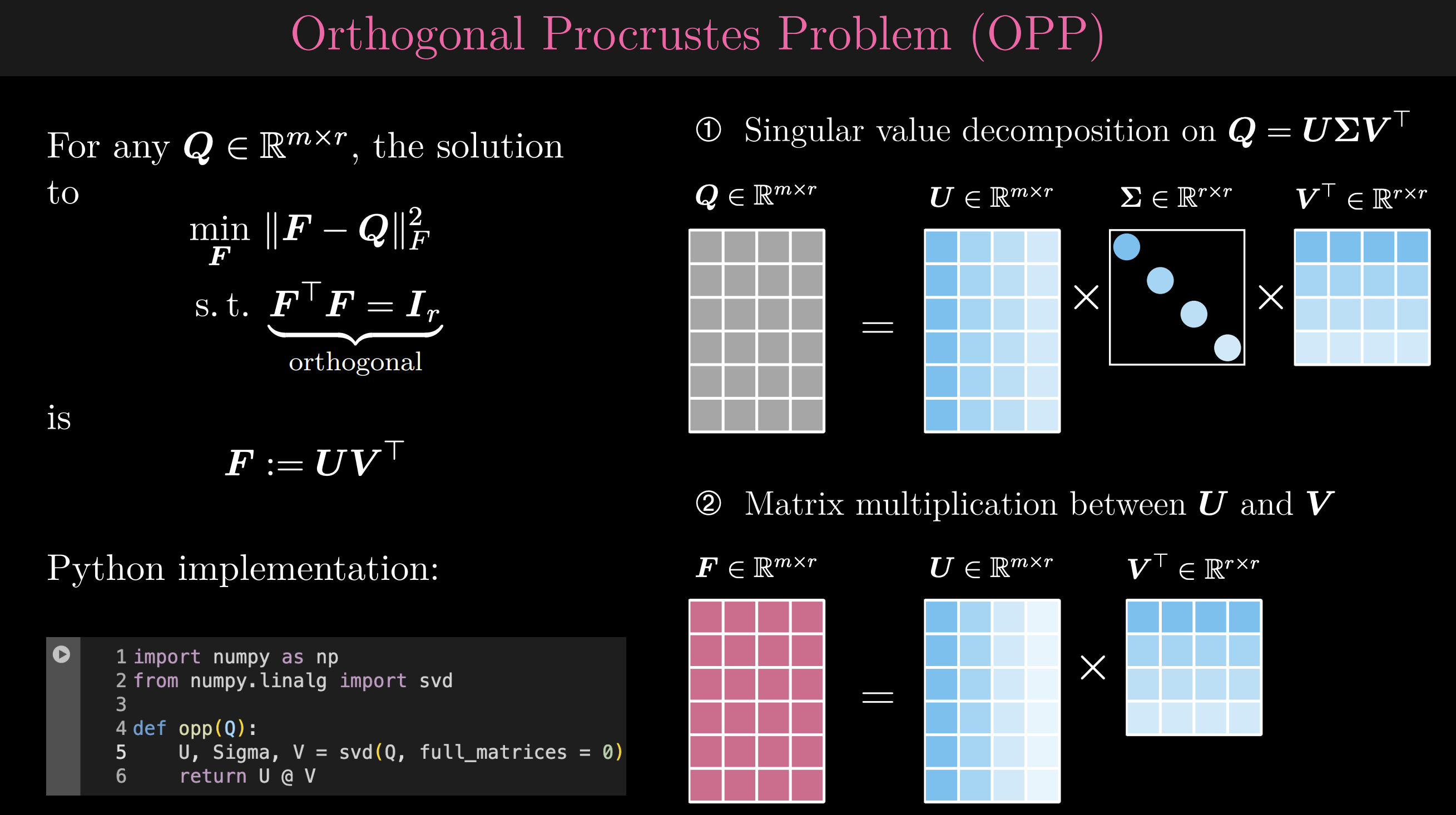
Orthogonal Procrustes Problem
Ever heard of the Orthogonal Procrustes Problem (OPP)? It might sound complex, but the optimal solution can be achieved in just two simple steps:
- Singular Value Decomposition (SVD)
- Matrix Multiplication
That’s it! This elegant approach helps find the closest orthogonal matrix to a given one, minimizing the Frobenius norm.
📌 Key Takeaways:
- OPP is a powerful tool for matrix alignment and optimization.
- The solution is computationally efficient with SVD at its core.
- Python makes implementation a breeze—just a few lines of code!
49th Commit
Amazon Deforestation
Deforestation in the Amazon: past, present and future visually analyzed the deforestation rates of recent years, identifying the main threats (e.g., cattle-raising activity, road network, and navigable rivers) in the present and pointing to measures needed to reverse this process. There are some basic data:
- In 2001, the forest cover of the Amazon occupied over 600 million hectares.
- Between 2001 and 2020, the deforestation in the Amazon totalled about 54.2 million hectares, the equivalent of 9% of the forest cover.
The Amazon could lose almost half of what it lost in the past two decades.
48th Commit
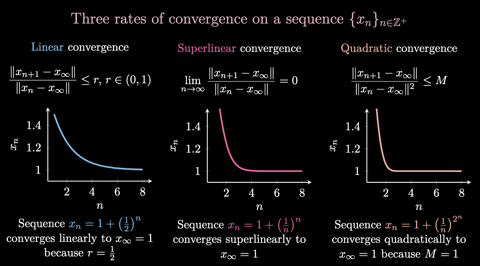
Convergence Rates
References
47th Commit
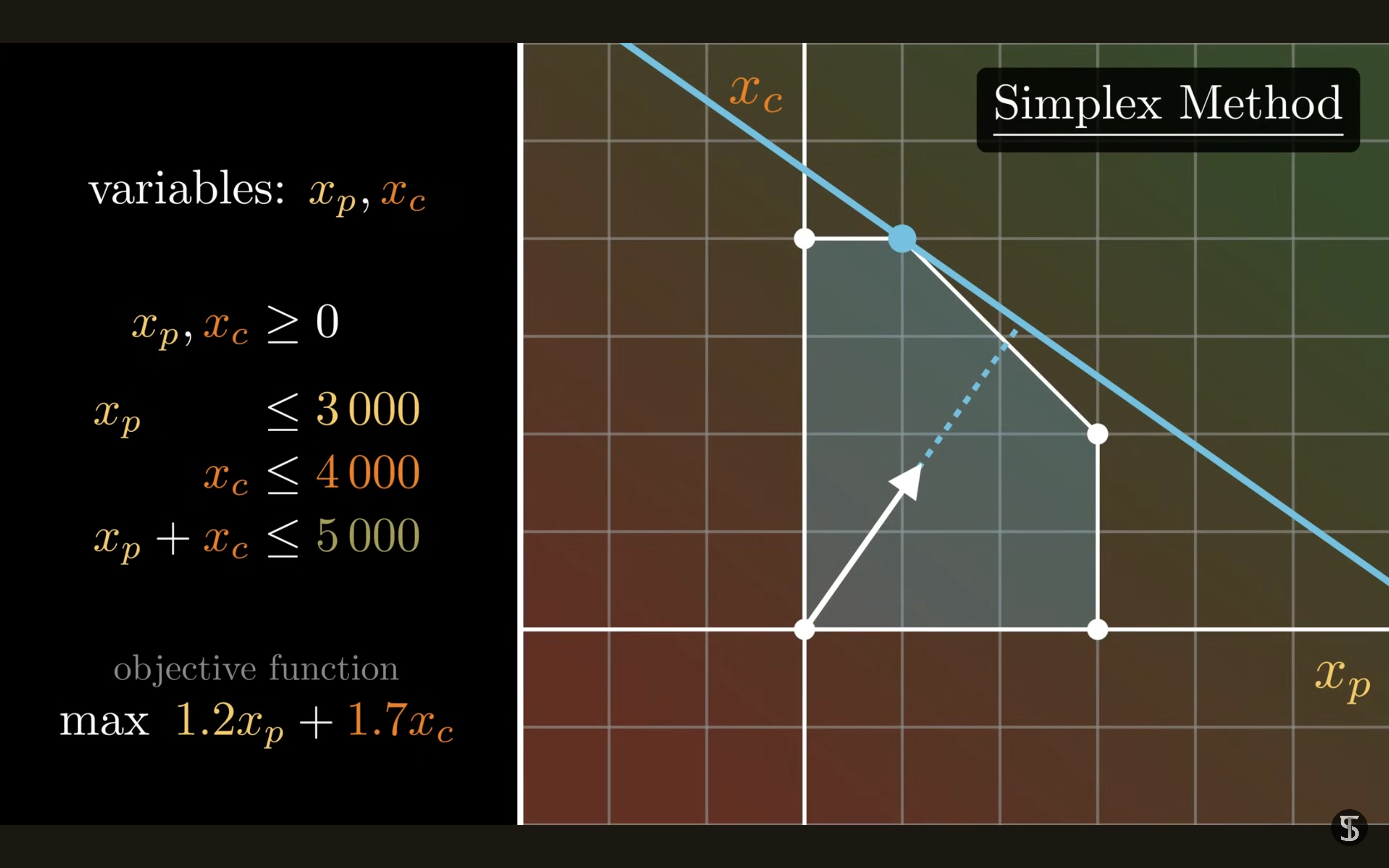
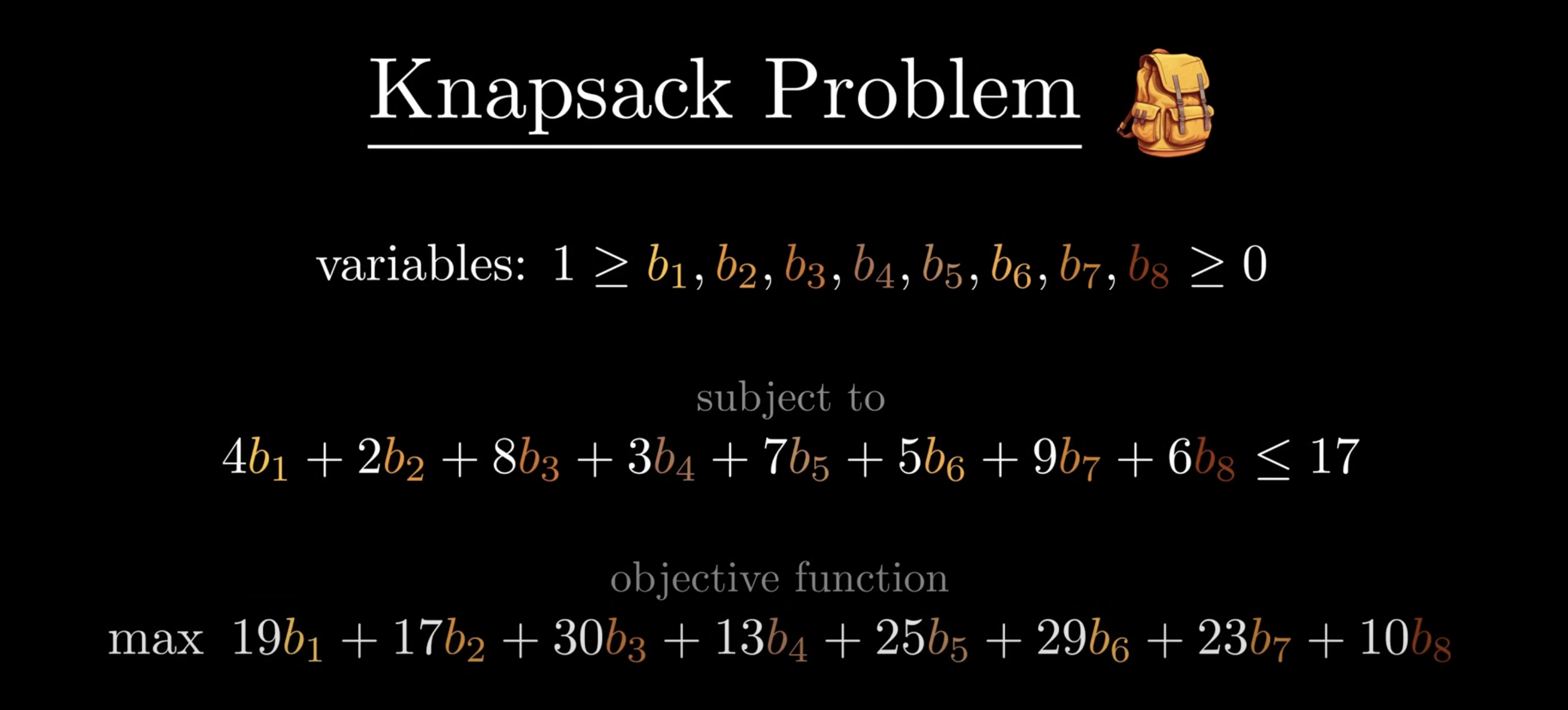
The Art of Linear Programming
Linear programming is an important technique for solving NP-hard problems such as Knapsack (e.g., packing problem), TSP, and Vertex Cover.
46th Commit
Semidefinite Programming
The basic definition of positive definite matrix is that: For any square matrix , if it always holds that
with any not being a vector of zeros, then
is a positive definite matrix. Similarly, we can define a positive semidefinite matrix as follows,
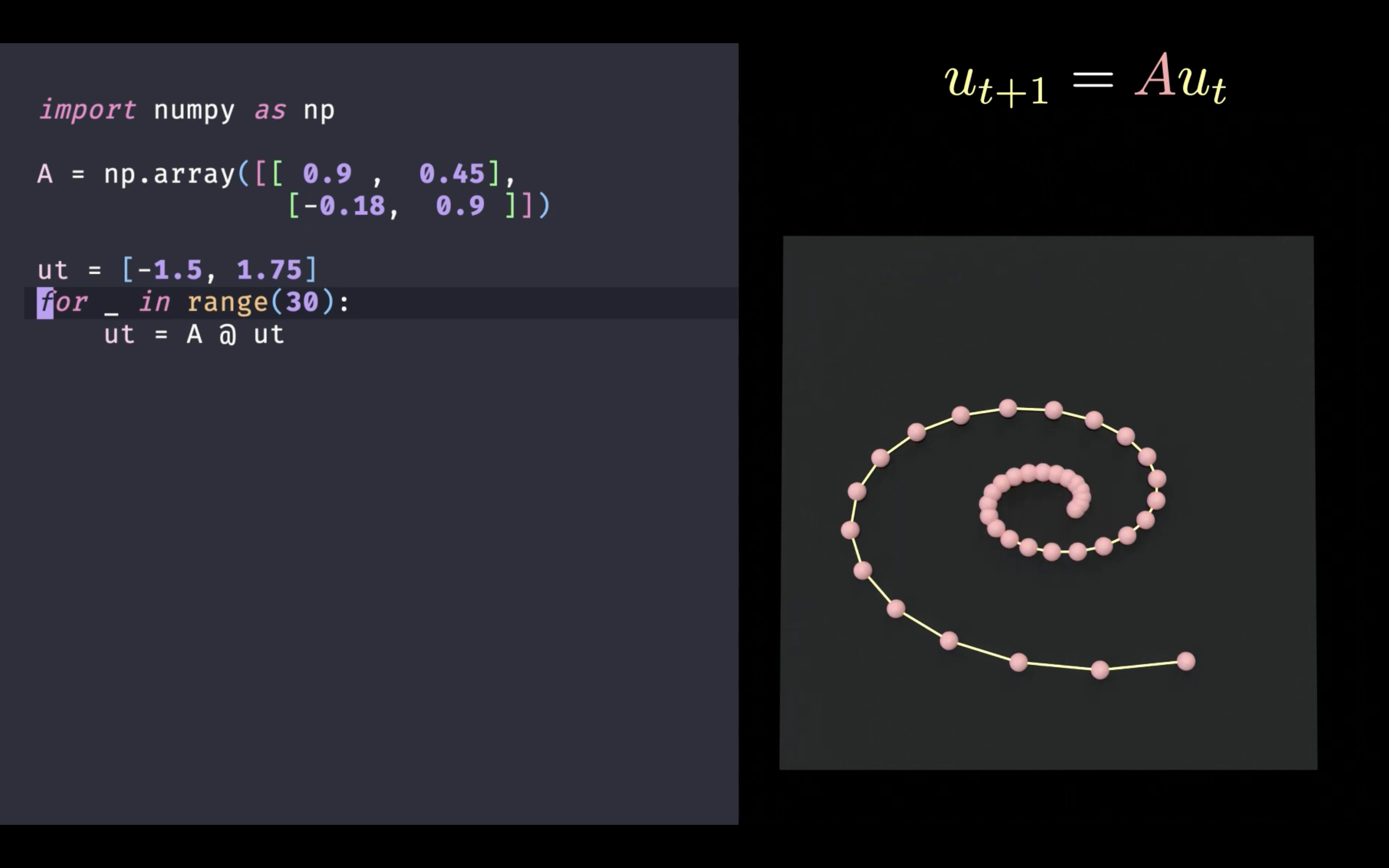
Semidefinite programming is the most exciting development of mathematical programming techniques in 1990s. One can leverage an initial point , following by the governing equation
, to build a dynamical system as shown below.
References
- What Does It Mean For a Matrix to be POSITIVE? The Practical Guide to Semidefinite Programming(1/4)
- The Practical Guide to Semidefinite Programming (2/4)
- Stability of Linear Dynamical Systems: The Practical Guide to Semidefinite Programming (3/4)
- Goemans-Williamson Max-Cut Algorithm: The Practical Guide to Semidefinite Programming (4/4)
45th Commit
Physics-Informed Machine Learning
Reviewed machine learning algorithms:
- Deterministic regression
- Linear regression
- Decision tree
- Machine learning algorithms: Sparse Identification of Nonlinear Dynamics (SINDy)
- Neural networks
- Probabilistic regression (Gaussian process regression)
- Ensemble methods
- Bagging (Random forest)
- Boosting (Gradient boosting machine, XGB regressor)
References
- Navid Zobeiry. Physics-Informed Machine Learning: A nine-lecture series on Physics-Informed Machine Learning (PIML) delivered by Professor Navid Zobeiry. This course introduces the key techniques of PIML and demonstrates how integrating physics-based constraints with machine learning (ML) can help solve complex multi-physics challenges in engineering.
44th Commit
Sparse Linear Regression
For any vector and matrix
, the sparse linear regression such that
There might be two solutions:
1) Mixed-integer programming such that
where is a sufficiently large constant.
2) Semidefinite programming such that
MIP provides exact solution, but it scales poorly with . SDP has better scalability, but not exact in most cases.
43rd Commit
Matrix Calculus for Machine Learning and Beyond
42nd Commit
Causal Inference, Causal Discovery, and Machine Learning
Causal inference is a framework to answer causal questions from observational and/or experimental data. It is important to infer underlying mechanisms of data (e.g., climate system), learn correlation networks, and recognize patterns. Pearl’s causal inference framework assumes an underlying structural causal model with an associated acyclic graph.
There are two types of tasks in the causal inference framework: 1) Utilizing qualitative causal knowledge in the form of directed acyclic graphs; 2) Learning causal graphs based on general assumption.
References
41st Commit
Composable Optimization for Robotic Motion Planning and Control
From a perspective of control as optimization, the objective could be what one wants system to do, given the model of one’s robot as constraints. This is exactly an optimal control problem such that
References
- MIT Robotics - Zac Manchester - Composable Optimization for Robotic Motion Planning and Control. YouTube.
40th Commit
Cauchy-Schwarz Regularizers
The main idea is that Cauchy-Schwarz inequality can be used to binarize neural networks. Cauchy-Schwarz regularizers are a new class of regularization that can promote discrete-valued vectors, eigenvectors of a given matrix, and orthogonal matrices. These regularizers are effective for quantizing neural network weights and solving underdetermined systems of linear equations.
References
- Sueda Taner, Ziyi Wang, Christoph Studer (2025). Cauchy-Schwarz Regularizers. ICLR 2025.
39th Commit
Nystrom Truncation of Spectral Features
Parameterizing policy gradient. (Mercer’s Theorem) If is a continuous, symmetric, and positive definite kernel, then there exists a sequence of non-negative eigenvalues
and corresponding orthonomal basis
such that
In practice, for large datasets, computing the full kernel matrix and its eigenvalue decomposition (EVD) is in
time and
memory.
The Nystrom method approximates the kernel matrix by selecting a subset. Let
be the
kernel matrix for the subset and
be the
kernel matrix between the full dataset and the subset, then the Nystrom approximation of
is
Furthermore, let be the EVD, then
corresponding to eigenvectors and eigenvalues. Selecting top- eigenvalues and eigenvectors, denoted by
and
, respectively. The truncation approximation of the kernel matrix becomes
References
- Na Li (Harvard). Representation-based Learning and Control for Dynamical Systems. YouTube.
38th Commit
Sparse Dictionary Learning
Interpretable machine learning provides a data-driven framework for understanding complicated dynamical systems. One important perspective is sparsity to reinforce the interpretability of several state-of-the-art models. Sparse dictionary learning stems from sparse signal processing, which takes the form of linear regression with sparse parameters.
In a very recent study, researchers developed an interpretable and efficient reinforcement learning model for sparse dictionary learning. The essential idea is iteratively improving control and dynamics on the data where
is the velocity matrix and
could be angles. Reinforcement learning can train policies in the dictionary approximation. However, one of the challenges is how to address the overfitting issue. In the modeling process, uncertainty quantification is also meaningful to improve the robustness of the system control.
References
- Nicholas Zolman, Urban Fasel, J. Nathan Kutz, Steven L. Brunton (2024). SINDy-RL: Interpretable and Efficient Model-Based Reinforcement Learning. arXiv:2403.09110.
37th Commit
Cardinality Minimization, Constraints, and Regularization
This is a review paper for solving the optimization problem that involves the cardinality of variable vectors in constraints or objective function. The problems can be formulated as follows,
- Cardinality minimization problems:
- Cardinality-constrained problems:
- Regularized cardinality problems:
These optimization problems have broad applications such as signal and image processing, portfolio selection, and machine learning.
References
- Andreas M. Tillmann, Daniel Bienstock, Andrea Lodi, Alexandra Schwartz (2024). Cardinality Minimization, Constraints, and Regularization: A Survey. SIAM Review, 66(3). [PDF]
36th Commit
Single-Factor Matrix Decomposition with Sparse Penalty
For any positive semidefinite matrix , the optimization problem of rank-one single-factor matrix decomposition with sparse penalty can be formulated as follows,
can be solved by the following algorithm:
- Initialize
as the unit vector with equal entries;
- Repeat
- Compute
- Until convergence
- Compute
(referring to the singular value);
- Compute
.
In the algorithm, the soft-thresholding operator is defined as
for all .
References
-
(Deng et al., 2021) Correlation tensor decomposition and its application in spatial imaging data. Journal of the American Statistical Association. [DOI] (see Algorithm 2)
-
(Witten et al., 2009) A penalized matrix decomposition, with applications to sparse principal components and canonical correlation analysis. Biostatistics. [DOI]
35th Commit
Iterative Shrinkage Thresholding Algorithm (ISTA)
In machine learning, the closed-form solution to LASSO is defined upon the soft thresholding operator such that
element-wise, we have
for all .
Considering the optimization problem
The proximal gradient update can be written as follows,
where is the step size, and the gradient of the first component in the objective function is
.
References
- Ryan Tibshirani. Proximal Gradient Descent (and Acceleration).
- Xiaohan Chen, Jialin Liu, Zhangyang Wang, Wotao Yin (2021). Hyperparameter Tuning is All You Need for LISTA. NeurIPS 2021.
34th Commit
Learning Sparse Nonparametric Directed Acyclic Graphs (DAG)
DAG learning problem: Given a data matrix consisting of
independent and identically distributed observations and
column vectors
, one can learn the DAG
that encodes the dependency between the variables in
. One approach is to learn
such that
using a well-designed score. Given a loss function
such as least squares or the negative log-likelihood, the optimization problem can be summarized as follows,
Two challenges in this formulation:
- How to enforce the acyclicity constraint that
?
- How to enforce sparsity in the learned DAG
?
If one uses MLP in the optimization, then it becomes
where denotes all parameters and the parameters of the
th MLP are
.
References
- Xun Zheng, Bryon Aragam, Pradeep Ravikumar, Eric P. Xing (2018). DAGs with NO TEARS: Continuous Optimization for Structure Learning. arXiv:1803.01422.
- Xun Zheng, Chen Dan, Bryon Aragam, Pradeep Ravikumar, Eric P. Xing (2019). Learning Sparse Nonparametric DAGs. arXiv:1909.13189.
- Victor Chernozhukov, Christian Hansen, Nathan Kallus, Martin Spindler, Vasilis Syrgkanis (2024). Applied Causal Inference Powered by ML and AI. arXiv:2403.02467. (See Chapter 7)
33rd Commit
Learning Sparse Nonlinear Dynamics via Mixed-Integer Optimization
Discovering governing equations of complex dynamical systems directly from data is a central problem in scientific machine learning. In recent years, the sparse identification of nonlinear dynamics (SINDy, see Brunton et al., (2016)) framework, powered by heuristic sparse regression methods, has become a dominant tool for learning parsimonious models. The optimization problem for learning system equations is
where are lower and upper bounds on the coefficients. The full system dynamics are
.
References
- Bertsimas, D., & Gurnee, W. (2023). Learning sparse nonlinear dynamics via mixed-integer optimization. Nonlinear Dynamics, 111(7), 6585-6604.
32nd Commit
- Behavioral changes during the COVID-19 pandemic decreased income diversity of urban encounters
- COVID-19 is linked to changes in the time–space dimension of human mobility
- Evacuation patterns and socioeconomic stratification in the context of wildfires in Chile
- Fine tune an LLM
- Learning with Combinatorial Optimization Layers: A Probabilistic Approach
31st Commit
 -Statistic & Student -Distribution
Given population mean , suppose the sample mean
, sample standard deviation
, and sample size
(small value), the formula of
-statistic for small sample sizes is written as follows,
A high absolute value of suggests a statistically significant difference.
is the null hypothesis, namely, the population mean is
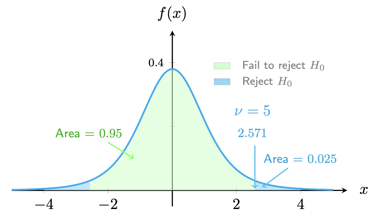
. Below is the student
-distribution with a
confidence interval.
Please check out the details of the relevance of -statistics for small sample sizes as the teaching sample.
Supporting Materials
- Hypothesis Testing Problems - Z Test & T Statistics - One & Two Tailed Tests 2
- Introduction to the t Distribution (non-technical)
- Confidence Intervals for One Mean: Determining the Required Sample Size
- Student’s T Distribution
- An Introduction to the t Distribution (Includes some mathematical details)
30th Commit
Interpretable ML vs. Explainable ML
In the context of AI, there is a subtle difference between terms interpretability and explainability. The interpretability techniques such as sparse linear regression were used to “understand how the underlying AI technology works”, while the explainability refer to “the level of understanding how AI-based systems produce with a given result”. Main claim from Wikipedia is that “treating the model as a black box and analyzing how marginal changes to the inputs affect the result sometimes provides a sufficient explanation.”
References
- Explainable Artificial Intelligence on Wikipedia.
- W. James Murdoch, Chandan Singh, Karl Kumbier, and Bin Yu (2019). Definitions, methods, and applications in interpretable machine learning. PNAS.
- Christoph Molnar (2024). Interpretable Machine Learning: A Guide for Making Black Box Models Explainable.
29th Commit
INFORMS 2024 | Optimal k-Sparse Ridge Regression
The classical linear regression with a -norm induced sparsity penalty can be written as follows,
which is equivalent to
References
- Jiachang Liu, Sam Rosen, Chudi Zhong, Cynthia Rudin (2023). OKRidge: Scalable Optimal k-Sparse Ridge Regression. NeurIPS 2023.
28th Commit
Mixed Integer Linear Programming (Example)
import cvxpy as cp
import numpy as np

# Data
n, d, k = 100, 50, 3  # n: samples, d: features, k: sparsity level
X = np.random.randn(n, d)
y = np.random.randn(n)
M = 1  # Large constant for enforcing non-zero constraint

# Variables
beta = cp.Variable(d, nonneg=True)
z = cp.Variable(d, boolean=True)

# Constraints
constraints = [
    cp.sum(z) <= k,
    beta <= M * z,
    beta >= 0
]

# Objective
objective = cp.Minimize(cp.sum_squares(y - X @ beta))

# Problem
problem = cp.Problem(objective, constraints)
problem.solve(solver=cp.GUROBI)  # Ensure to use a solver that supports MIP

# Solution
print("Optimal beta:", beta.value)
print("Active indices:", np.nonzero(z.value > 0.5)[0])
Note that the “Model too large for size-limited Gurobi license” error.
27th Commit
Importance of Sparsity in Interpretable Machine Learning
Sparsity is an important type of model-based interpretability methods. Typically, the practitioner can impose sparsity on the model by limiting the number of nonzero parameters. When the number of nonzero parameters is sufficiently small, a practitioner can interpret the variables corresponding to those parameters as being meaningfully related to the outcome in question and can also interpret the magnitude and direction of the parameters. Two important methods including -norm penalty (e.g., LASSO) and
-norm constraint (e.g., OMP). Model sparsity is often useful for high-dimensional problems, where the goal is to identify key features for further analysis.
References
- W. James Murdoch, Chandan Singh, Karl Kumbier, Reza Abbasi-Asl, and Bin Yu (2019). Definitions, methods, and applications in interpretable machine learning. PNAS.
26th Commit
INFORMS 2024 | Core Tensor Shape Optimization
Recall that the sum of squared singular values of and outcomes
is
because Frobenius norm is invariant under orthogonal transformations with respect to singular vectors.
This means that we can solve a singular value packing problem instead of considering the complement of the surrogate loss. Please reproduce the aforementioned property as follows,
import numpy as np

X = np.random.rand(100, 100)
print(np.linalg.norm(X, 'fro') ** 2)
u, s, v = np.linalg.svd(X, full_matrices = False)
print(np.linalg.norm(s, 2) ** 2)
Thus, Tucker packing problem on the non-increasing sequences (w.r.t. singular values), the optimization problem is given by
The optimization problem can be implemented by using an integer programming solvers, and its solution quality is competitive with the greedy algorithm.
References
- Mehrdad Ghadiri, Matthew Fahrbach, Gang Fu, Vahab Mirrokni (2023). Approximately Optimal Core Shapes for Tensor Decompositions. ICML 2023. [Python code]
25th Commit
Mobile Service Usage Data
- Orlando E. Martínez-Durive et al. (2023). The NetMob23 Dataset: A High-resolution Multi-region Service-level Mobile Data Traffic Cartography. arXiv:2305.06933.
- André Zanella (2024). Characterizing Large-Scale Mobile Traffic Measurements for Urban, Social and Networks Sciences. PhD thesis.
24th Commit
Optimization in Reinforcement Learning
References
- Jalaj Bhandari and Daniel Russo (2024). Global Optimality Guarantees for Policy Gradient Methods. Operations Research, 72(5): 1906 - 1927.
- Lucia Falconi, Andrea Martinelli, and John Lygeros (2024). Data-driven optimal control via linear programming: boundedness guarantees. IEEE Transactions on Automatic Control.
23rd Commit
Sparse and Time-Varying Regression
This work addresses a time series regression problem for features and outcomes
, taking the following expression:
where are coefficient vectors, which are supposed to represent both sparsity and time-varying behaviors of the system. Thus, the optimization problem has both temporal smoothing (in the objective) and sparsity (in the constraint), e.g.,
where the constraint is indeed the -norm of vectors, as the symbol
denotes the index set of nonzero entries in the vector. For instance, the first constraint can be rewritten as
. Thus,
stand for sparsity levels.
The methodological contribution is reformulating this problem as a binary convex optimization problem (w/ a novel relaxation of the objective function), which can be solved efficiently using a cutting plane-type algorithm.
References
- Dimitris Bertsimas, Vassilis Digalakis, Michael Lingzhi Li, Omar Skali Lami (2024). Slowly Varying Regression Under Sparsity. Operations Research. [arXiv]
22nd Commit
Revisiting  -Norm Minimization
References
- Lijun Ding (2023). One dimensional least absolute deviation problem. Blog post.
- Gregory Gundersen (2022). Weighted Least Squares. Blog post.
- stephentu’s blog (2014). Subdifferential of a norm. Blog post.
21st Commit
Research Seminars
- Computational Research in Boston and Beyond (CRIBB) seminar series: A forum for interactions among scientists and engineers throughout the Boston area working on a range of computational problems. This forum consists of a monthly seminar where individuals present their work.
- Param-Intelligence (𝝅) seminar series: A dynamic platform for researchers, engineers, and students to explore and discuss the latest advancements in integrating machine learning with scientific computing. Key topics include data-driven modeling, physics-informed neural surrogates, neural operators, and hybrid computational methods, with a strong focus on real-world applications across various fields of computational science and engineering.
20th Commit
Robust, Interpretable Statistical Models: Sparse Regression with the LASSO
First of all, we revisit the classical least squares such that
Putting the Tikhonov regularization together with least squares, it refers to as the Ridge regression used almost everywhere:
Another classical variant is the LASSO:
with -norm on the vector
. It allows one to find a few columns of the matrix
that are most correlated with the designed outcomes (e.g.,
) for making decisions (e.g., why they take actions?).
One interesting application is using sparsity-promoting techniques and machine learning with nonlinear dynamical systems to discover governing equations from noisy measurement data. The only as-sumption about the structure of the model is that there are only a fewimportant terms that govern the dynamics, so that the equations aresparse in the space of possible functions; this assumption holds formany physical systems in an appropriate basis.
References
- Steve Brunton (2021). Robust, Interpretable Statistical Models: Sparse Regression with the LASSO. see YouTube. (Note: Original paper by Tibshirani (1996))
- Steve L. Brunton, Joshua L. Proctor, and Nathan Kutz (2016). Discovering governing equations from data by sparse identification of nonlinear dynamical systems. Proceedings of the National Academy of Sciences. 113 (15), 3932-3937.
19th Commit
Causal Inference for Geosciences
Learning causal interactions from time series of complex dynamical systems is of great significance in real-world systems. But the questions arise as: 1) How to formulate causal inference for complex dynamical systems? 2) How to detect causal links? 3) How to quantify causal interactions?
References
- Jakob Runge (2017). Causal inference and complex network methods for the geosciences. Slides.
- Jakob Runge, Andreas Gerhardus, Gherardo Varando, Veronika Eyring & Gustau Camps-Valls (2023). Causal inference for time series. Nature Reviews Earth & Environment, 4: 487–505.
- Jitkomut Songsiri (2013). Sparse autoregressive model estimation for learning Granger causality in time series. 2013 IEEE International Conference on Acoustics, Speech and Signal Processing.
18th Commit
Tensor Factorization for Knowledge Graph Completion
Knowledge graph completion is a kind of link prediction problems, inferring missing “facts” based on existing ones. Tucker decomposition of the binary tensor representation of knowledge graph triples allows one to make data completion.
References
- TuckER: Tensor Factorization for Knowledge Graph Completion. GitHub.
- Ivana Balazevic, Carl Allen, Timothy M. Hospedales (2019). TuckER: Tensor Factorization for Knowledge Graph Completion. arXiv:1901.09590. [PDF]
17th Commit
RESCAL: Tensor-Based Relational Learning
Multi-relational data is everywhere in real-world applications such as computational biology, social networks, and semantic web. This type of data is often represented in the form of graphs or networks where nodes represent entities, and edges represent different types of relationships.
Instead of using the classical Tucker and CP tensor decomposition, RESCAL takes the inherent structure of dyadic relational data into account, whose tensor factorization on the tensor variable (i.e., frontal tensor slices) is
where is the global entity factor matrix, and
specifies the interaction of the latent components. Such kind of methods can be used to solve link prediction, collective classification, and link-based clustering.
References
- Maximilian Nickel, Volker Tresp, Hans-Peter Kriegel (2011). A Three-Way Model for Collective Learning on Multi-Relational Data. ICML 2011. [PDF] [Slides]
- Maximilian Nickel (2013). Tensor Factorization for Relational Learning. PhD thesis.
- Denis Krompaß, Maximilian Nickel, Xueyan Jiang, Volker Tresp (2013). Non-Negative Tensor Factorization with RESCAL. ECML Workshop 2013.
- Elynn Y. Chen, Rong Chen (2019). Modeling Dynamic Transport Network with Matrix Factor Models: with an Application to International Trade Flow. arXiv:1901.00769. [PDF]
- Zhanhong Cheng. factor_matrix_time_series. GitHub.
16th Commit
Subspace Pursuit Algorithm
Considering the optimization problem for estimating -sparse vector
:
with the signal vector (or measurement vector), the dictionary matrix
(or measurement matrix), and the sparsity level
.
The subspace pursuit algorithm, introduced by W. Dai and O. Milenkovic
in 2008, is a classical algorithm in the greedy family. It bears some resemblance with compressive sampling matching
pursuit (CoSaMP by D. Needell and J. A. Tropp in 2008), except that, instead of , only
indices of largest (in modulus) entries of the residual vector are selected, and that an additional orthogonal projection step is performed at each iteration. The implementation of subspace pursuit algorithm (adapted from A Mathematical Introduction to Compressive Sensing, see Page 65) can be summarized as follows:
- Input: Signal vector
, dictionary matrix
, and sparsity level
.
- Output:
-sparse vector
and index set
.
- Initialization: Sparse vector
(i.e., zero vector), index set
(i.e., empty set), and error vector
.
- while not stop do
- Find
as the index set of the
.
.
(least squares).
- Find
.
- Set
for all
.
.
- Find
- end
The subspace pursuit algorithm is a fixed-cardinality method, quite different from the classical orthogonal matching pursuit algorithm developed in 1993 such that
- Input: Signal vector
- Output:
- Initialization: Sparse vector
- while not stop do
- Find
.
- Find
- end
15th Commit
Synthetic Sweden Mobility
The Synthetic Sweden Mobility (SySMo) model provides a simplified yet statistically realistic microscopic representation of the real population of Sweden. The agents in this synthetic population contain socioeconomic attributes, household characteristics, and corresponding activity plans for an average weekday. This agent-based modelling approach derives the transportation demand from the agents’ planned activities using various transport modes (e.g., car, public transport, bike, and walking). The dataset is available on Zenodo.
Going back to the individual mobility trajectory, there would be some opportunities to approach taxi trajectory data such as
- 1 million+ trips collected by 13,000+ taxi cabs during 5 days in Harbin, China
- Daily GPS trajectory data of 664 electric taxis in Shenzhen, China
- Takahiro Yabe, Kota Tsubouchi, Toru Shimizu, Yoshihide Sekimoto, Kaoru Sezaki, Esteban Moro & Alex Pentland (2024). YJMob100K: City-scale and longitudinal dataset of anonymized human mobility trajectories. Scientific Data. [Data] [Challenge]
- The dataset comprises trajectory data of traffic participants, along with traffic light data, current local weather data, and air quality data from the Application Platform Intelligent Mobility (AIM) Research Intersection
14th Commit
Prediction on Extreme Floods
AI increases global access to reliable flood forecasts (see dataset).
Another weather forecasting dataset for consideration: Rain forecasts world-wide on an expansive data set with over a magnitude more hi-res rain radar data.
References
- Nearing, G., Cohen, D., Dube, V. et al. (2024). Global prediction of extreme floods in ungauged watersheds. Nature, 627: 559–563.
13th Commit
Sparse Recovery Problem
Considering a general optimization problem for estimating the sparse vector :
with the signal vector and a dictionary of elementary functions
(i.e., dictionary matrix). There are a lot of solution algorithms in literature:
- Mehrdad Yaghoobi, Di Wu, Mike E. Davies (2015). Fast Non-Negative Orthogonal Matching Pursuit. IEEE Signal Processing Letters, 22 (9): 1229-1233.
- Thanh Thi Nguyen, Jérôme Idier, Charles Soussen, El-Hadi Djermoune (2019). Non-Negative Orthogonal Greedy Algorithms. IEEE Transactions on Signal Processing, 67 (21): 5643-5658.
- Nicolas Nadisic, Arnaud Vandaele, Nicolas Gillis, Jeremy E. Cohen (2020). Exact Sparse Nonnegative Least Squares. IEEE International Conference on Acoustics, Speech and Signal Processing (ICASSP).
- Chiara Ravazzi, Francesco Bullo, Fabrizio Dabbene (2022). Unveiling Oligarchy in Influence Networks From Partial Information. IEEE Transactions on Control of Network Systems, 10 (3): 1279-1290.
- Thi Thanh Nguyen (2019). Orthogonal greedy algorithms for non-negative sparse reconstruction. PhD thesis.
The most classical (greedy) method for solving the linear sparse regression is orthogonal matching pursuit (see an introduction here).
12th Commit
Economic Complexity
References
- César A. Hidalgo (2021). Economic complexity theory and applications. Nature Reviews Physics. 3: 92-113.
11th Commit
Time-Varying Autoregressive Models
Vector autoregression (VAR) has a key assumption that the coeffcients are invariant across time (i.e., time-invariant), but it is not always true when accounting for psychological phenomena such as the phase transition from a healthy to unhealthy state (or vice versa). Consequently, time-varying vector autoregressive models are of great significance for capturing the parameter changes in response to interventions. From the statistical perspective, there are two types of lagged effects between pairs of variables: autocorrelations (e.g., ) and cross-lagged effects (e.g.,
). The time-varying autoregressive models can be solved by using generalized additive model and kernel smoothing estimation.
References
- Haslbeck, J. M., Bringmann, L. F., & Waldorp, L. J. (2021). A tutorial on estimating time-varying vector autoregressive models. Multivariate Behavioral Research, 56(1), 120-149.
10th Commit
Higher-Order Graph & Hypergraph
The concept of a higher-order graph extends the traditional notion of a graph, which consists of nodes and edges, to capture more complex relationships and structures in data. A common formalism for representing higher-order graphs is through hypergraphs, which generalize the concept of a graph to allow for hyperedges connecting multiple nodes. In a hypergraph, each hyperedge connects a subset of nodes, forming higher-order relationships among them.
References
- Higher-order organization of complex networks. Stanford University.
- Quintino Francesco Lotito, Federico Musciotto, Alberto Montresor, Federico Battiston (2022). Higher-order motif analysis in hypergraphs. Communications Physics, volume 5, Article number: 79.
- Christian Bick, Elizabeth Gross, Heather A. Harrington, and Michael T. Schaub (2023). What are higher-order networks? SIAM Review. 65(3).
- Vincent Thibeault, Antoine Allard & Patrick Desrosiers (2024). The low-rank hypothesis of complex systems. Nature Physics. 20: 294-302.
- Louis Boucherie, Benjamin F. Maier, Sune Lehmann (2024). Decomposing geographical and universal aspects of human mobility. arXiv:2405.08746.
- Raissa M. D’Souza, Mario di Bernardo & Yang-Yu Liu (2023). Controlling complex networks with complex nodes. Nature Reviews Physics. 5: 250–262.
- PS Chodrow, N Veldt, AR Benson (2021). Generative hypergraph clustering: From blockmodels to modularity. Science Advances, 28(7).
9th Commit
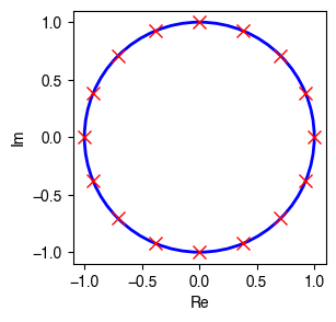
Eigenvalues of Directed Cycles
The graph signal processing possesses an interesting property of directed cycle (see Figure 2 in the literature). The adjacency matrix of a directed cycle has a set of unit eigenvalues as follows.
import numpy as np

## Construct an adjacency matrix A
a = np.array([0, 1, 0, 0, 0, 0, 0, 0, 0, 0, 0, 0, 0, 0, 0, 0])
n = a.shape[0]
A = np.zeros((n, n))
A[:, 0] = a
for i in range(1, n):
    A[:, i] = np.append(a[-i :], a[: -i])

## Perform eigenvalue decomposition on A
eig_val, eig_vec = np.linalg.eig(A)

## Plot eigenvalues
import matplotlib.pyplot as plt
plt.rcParams['font.family'] = 'Helvetica'

fig = plt.figure(figsize = (3, 3))
ax = fig.add_subplot(1, 1, 1)
circ = plt.Circle((0, 0), radius = 1, edgecolor = 'b', facecolor = 'None', linewidth = 2)
ax.add_patch(circ)
plt.plot(eig_val.real, eig_val.imag, 'rx', markersize = 8)
ax.set_aspect('equal', adjustable = 'box')
plt.xlabel('Re')
plt.ylabel('Im')
plt.show()
fig.savefig('eigenvalues_directed_cycle.png', bbox_inches = 'tight')
8th Commit
Graph Filter
Defining graph-aware operator plays an important role for characterizing a signal with
vertices over a graph
. One simple idea is introducing the adjacency matrix
so that the operation is
. In that case,
is a simple operator that accounts for the local connectivity of
. One example is using the classical unit delay (seems to be time-shift) such that
The simplest signal operation as multiplication by the adjacency matrix defines graph filters as matrix polynomials of the form
For instance, we have
On the signal , it always holds that
When applying the polynomial filter to a graph signal , the operation
takes a local linear combination of the signal values at one-hop neighbors.
takes a local linear combination of
, referring to two-hop neighbors. Consequently, a graph filter
of order
represents the mixing values that are at most
hops away.
References
- Geert Leus, Antonio G. Marques, José M. F. Moura, Antonio Ortega, David I Shuman (2023). Graph Signal Processing: History, Development, Impact, and Outlook. arXiv:2303.12211.
- A Sandryhaila, JMF Moura (2013). Discrete signal processing on graphs: Graph filters. Section 3: Graph Filters.
- Henry Kenlay, Dorina Thanou, Xiaowen Dong (2020). On The Stability of Polynomial Spectral Graph Filters. ICASSP 2020.
- Xiaowen Dong, Dorina Thanou, Michael Rabbat, and Pascal Frossard (2019). Learning Graphs From Data: A signal representation perspective. IEEE Signal Processing Magazine.
- Eylem Tugçe Güneyi, Berkay Yaldız, Abdullah Canbolat, and Elif Vural (2024). Learning Graph ARMA Processes From Time-Vertex Spectra. IEEE Transactions on Signal Processing, 72: 47 - 56.
7th Commit
Graph Signals
For any graph where
is a finite set of
vertices, and
is the set of edges. Graph signals can be formally represented as vectors
where
(or say
in the following) stores the signal value at the
th vertex in
. The graph Fourier transform of
is element-wise defined as follows,
or another form such that
where consists of the eigenvectors
. The notation
is the conjugate of complex values, and
is the conjugate transpose.
The above graph Fourier transform can also be generalized to the graph signals in the form of multivariate time series. For instance, on the data , we have
where consists of the eigenvectors of the graph Laplacian matrix.
References
- Santiago Segarra, Weiyu Huang, and Alejandro Ribeiro (2020). Signal Processing on Graphs.
- Matthew Begue. Fourier analysis on graphs. Slides.
6th Commit
Graph Signal Processing
Graph signal processing not only focuses on the graph typology (e.g., connection between nodes), but also covers the quantity of nodes (i.e., graph signals) with weighted adjacency information.
References
- Antonio Ortega, Pascal Frossard, Jelena Kovacevic, Jose M. F. Moura, Pierre Vandergheynst (2017). Graph Signal Processing: Overview, Challenges and Applications. arXiv:1712.00468.
- Gonzalo Mateos, Santiago Segarra, Antonio G. Marques, Alejandro Ribeiro (2019). Connecting the Dots: Identifying Network Structure via Graph Signal Processing. IEEE Signal Processing Magazine. 36 (3): 16-43.
- Xiaowen Dong, Dorina Thanou, Laura Toni, Michael Bronstein, and Pascal Frossard (2020). Graph signal processing for machine learning: A review and new perspectives. arXiv:2007.16061. [Slides]
- Michael M. Bronstein, Joan Bruna, Taco Cohen, Petar Veličković (2021). Geometric Deep Learning: Grids, Groups, Graphs, Geodesics, and Gauges. arXiv:2104.13478.
- Wei Hu, Jiahao Pang, Xianming Liu, Dong Tian, Chia-Wen Lin, Anthony Vetro (2022). Graph Signal Processing for Geometric Data and Beyond: Theory and Applications. IEEE Transactions on Multimedia, 24: 3961-3977.
- Geert Leus, Antonio G. Marques, José M. F. Moura, Antonio Ortega, David I Shuman (2023). Graph Signal Processing: History, Development, Impact, and Outlook. arXiv:2303.12211.
- Spectral graph theory for dummies. YouTube.
5th Commit
Clifford Product
In Grassmann algebra, the inner product between two vectors and
(w/ basis vectors
and
) is given by
implies to be the multiplication between the magnitude of and the projection of
on
. Here, the notation
refers to the
norm, or say the magnitude.
is the angle between
and
in the plane containing them.
In contrast, the outer product (usually called Wedge product) is
implies to be the multiplication between and the projection of
on the orthogonal direction of
. Here, the unit bivector
represents the orientation (
or
) of the hyperplane of
(see Section II in geometric-algebra adaptive filters).
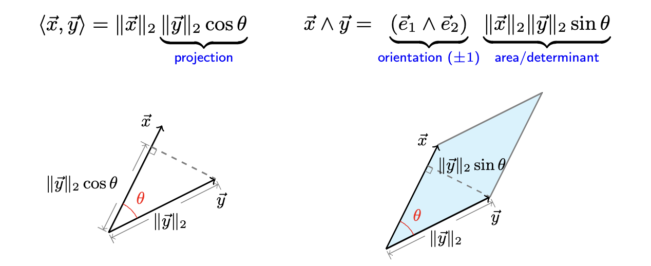
As a result, they consist of Clifford product (or called geometric product, denoted by the symbol ) such that
In particular, Clifford algebra is important for modeling vector fields, thus demonstrating valuable applications to wind velocity and fluid dynamics (e.g., Navier-Stokes equation).
References
- Spinors for Beginners 11: What is a Clifford Algebra? (and Geometric, Grassmann, Exterior Algebras). YouTube.
- A Swift Introduction to Geometric Algebra. YouTube.
- Learning on Graphs & Geometry. Weekly reading groups every Monday at 11 am ET.
- What’s the Clifford algebra? Mathematics stackexchange.
- Introducing CliffordLayers: Neural Network layers inspired by Clifford / Geometric Algebras. Microsoft Research AI4Science.
- David Ruhe, Jayesh K. Gupta, Steven de Keninck, Max Welling, Johannes Brandstetter (2023). Geometric Clifford Algebra Networks. arXiv:2302.06594.
- Maksim Zhdanov, David Ruhe, Maurice Weiler, Ana Lucic, Johannes Brandstetter, Patrick Forre (2024). Clifford-Steerable Convolutional Neural Networks. arXiv:2402.14730.
4th Commit
Bayesian Variable Selection
In genetic fine mapping, one critical problem is the variable selection in linear regression. There is a Bayesian variable selection based on the sum of single effects, i.e., the vector with one non-zero element. Given any data (of
explanatory variables) and
, one can build an optimization problem as follows,
where (
) is predefined by the number of correlated variables. The vectors
are the coefficients in this linear regression. This optimization problem can also be written as follows,
Or see Figure 1.1 in Section 1.1 Non-negative sparse reconstruction (Page 2) for an illustration.
References
- Gao Wang, Abhishek Sarkar, Peter Carbonetto and Matthew Stephens (2020). A simple new approach to variable selection in regression, with application to genetic fine mapping. Journal of the Royal Statistical Society Series B: Statistical Methodology, 82(5), 1273-1300.
- Emil Uffelmann, Qin Qin Huang, Nchangwi Syntia Munung, Jantina de Vries, Yukinori Okada, Alicia R. Martin, Hilary C. Martin, Tuuli Lappalainen & Danielle Posthuma (2021). Genome-wide association studies. Nature Reviews Methods Primers. 1: 59.
3rd Commit
Causal Effect Estimation/Imputation
The causal effect estimation problem is usually defined as a matrix completion on the partially observed matrix in which
units and
periods are involved. The observed index set is denoted by
. The optimization is from the classical matrix factorization techniques for recommender systems (see Koren et al.’09):
where and
are factor matrices, referring to units and periods, respectively. Here,
and
are bias vectors, corresponding to
units and
periods, respectively. This idea has also been examined on the tensor factorization (to be honest, performance gains are marginal), see e.g., Bayesian augmented tensor factorization by Chen et al.’19. In the causal effect imputation, one great challenge is how to handle the structural patterns of missing data as mentioned by Athey et al.’21. The structural missing patterns have been discussed on spatiotemporal data with autoregressive tensor factorization (for spatiotemporal predictions).
2nd Commit
Data Standardization in Healthcare
The motivation for discussing the value of standards for health datasets is the risk of algorithmic bias, consequently leading to the possible healthcare inequity. The problem arises from the systemic inequalities in the dataset curation and the unequal opportunities to access the data and research. The aim is to expolore the standards, frameworks, and best practices in health datasets. Some discrete insights throughout the whole paper are summarized as follows,
- AI as a medical device (AIaMD). One concern is the risk of systemic algorithmic bias (well-recognized in the literature) if models are trained on biased training datasets.
- Less accurate performance in certain patient groups when using the biased algorithms.
- Data diversity (Mainly discuss “how to improve”):
- Challenges: lack of standardization across attribute categories, difficulty in harmonizing several methods of data capture and data-governance restrictions.
- Inclusiveness is a core tenet of ethical AI in healthcare.
- Guidance on how to apply the principles in the curation (e.g., developing the data collection strategy), aggregation and use of health data.
- The use of metrics (measuring diversity). How to promote diversity and transparency?
- Future actions: Guidelines for data collection, handling missing data and labeling data.
References
- Anmol Arora, Joseph E. Alderman, Joanne Palmer, Shaswath Ganapathi, Elinor Laws, Melissa D. McCradden, Lauren Oakden-Rayner, Stephen R. Pfohl, Marzyeh Ghassemi, Francis McKay, Darren Treanor, Negar Rostamzadeh, Bilal Mateen, Jacqui Gath, Adewole O. Adebajo, Stephanie Kuku, Rubeta Matin, Katherine Heller, Elizabeth Sapey, Neil J. Sebire, Heather Cole-Lewis, Melanie Calvert, Alastair Denniston, Xiaoxuan Liu (2023). The value of standards for health datasets in artificial intelligence-based applications. Nature Medicine, 29: 2929–2938.
1st Commit
Large Time Series Forecasting Models
As we know, the training data in the large time series model is from different areas, this means that the model training process highly depends on the selected datasets across various areas, so one question is how to reduce the model biases if we consider the forecasting scenario as traffic flow or human mobility? Because I guess time series data in different areas should demonstrate different data behaviors. Hopefully, it is interesting to develop domain-specific time series datasets (e.g., Largest multi-city traffic dataset) and large models (e.g., TimeGPT).
References
- Gerald Woo, Chenghao Liu, Akshat Kumar, Caiming Xiong, Silvio Savarese, Doyen Sahoo (2024). Unified Training of Universal Time Series Forecasting Transformers. arXiv:2402.02592.
Motivation & Principle: “不积硅步,无以至千里。” (Small Steps to Accuracy)