Visualizing Germany Energy Consumption Data in Python

The analysis of energy consumption for future energy systems requires appropriate data. In the latest JERICHO-E-usage dataset, comprehensive data on useful energy consumption patterns for heat, cold, mechanical energy, information and communication, and light in high spatial and temporal resolution are available. The data are aggregated to the NUTS2 level, consisting of 38 regions in Germany.

Download Shapefile in the NUTS2 Level

Germany energy consumption data is a publicly available dataset. To visualize geographical distribution of these energy consumption data, we need to find appropriate .shp file and project data on it. We download the .shp from GISCO statistical unit dataset. In the download page, we set the following options:

Year: NUTS 2016
File format: SHP
Geometry type: Polygons (RG)
Scale: 03M
Coordinate reference system: EPSG: 4326

Then we can download the .shp file. In Python, geopandas is a powerful tool for visualizing geospatial data. It is not hard to use geopandas to visualize our data file.

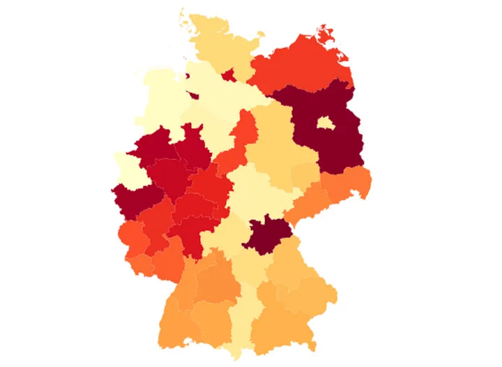
Figure 1. Geographical distribution of 38 regions in the NUTS2 level of Germany.

To draw Figure 1, please try the following Python codes. Note that two necessary packages include geopandas and matplotlib.

import geopandas as gpd
import matplotlib.pyplot as plt

fig = plt.figure(figsize = (14, 8))
ax = fig.subplots(1)
shape = gpd.read_file("NUTS_RG_03M_2016_4326.shp")
shape_de = shape[(shape['CNTR_CODE'] == 'DE') & (shape['LEVL_CODE'] == 2)]
shape_de.plot(cmap = 'YlOrRd_r', ax = ax)
plt.xticks([])
plt.yticks([])
for _, spine in ax.spines.items():
    spine.set_visible(False)
plt.show()

About the Dataset

The JERICHO-E-usage dataset provides the energy consumption of Germany in the whole year of 2019 (Priesmann et al., 2021). The dataset is spatially resolved at the NUTS2 level comprising 38 regions and temporally resolved in hours. The dataset distinguished among four sectors, namely, the residential, the industrial, the commerce, and the mobility sectors. Useful energy types comprise space heating, warm water, process heating, space cooling, process cooling, mechanical energy, information and communication technology, and lightning.

For the following analysis, we take into account the energy data of space heating of residential sectors. The data is of size 38-by-8760 in which 38 rows refer to the 38 regions in Germany and 8760 columns refer to the number of hours in 2019. As shown in Figure 1, it visualizes the geographical distribution of space heating consumption in Germany. The red regions show strong energy consumption, while the yellow regions show relatively weak energy consumption.

The original dataset is publicly available at here. We adapt the energy consumption data and .shp file in our GitHub repository.

Data Visualization

To visualize the energy consumption data on the road map, we should project the energy data onto the .shp file. In this story, we aggregate the total energy consumption in each season and then plot (four) subfigures for four seasons in 2019 (see Figure 2).

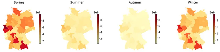
Figure 2. Geographical distribution of seasonal energy consumption of 2019 in Germany.

As shown in Figure 2, the space heating consumption are significantly reduced in Summer and Autumn, but it recovers to the Spring’s level in Winter. To draw this figure, please try the following Python codes.

import pandas as pd
import numpy as np
import geopandas as gpd
import matplotlib.pyplot as plt

# Upload shapefile
shape = gpd.read_file("NUTS_RG_03M_2016_4326.shp")
shape_de = shape[(shape['CNTR_CODE'] == 'DE') & (shape['LEVL_CODE'] == 2)]

# Upload energy data
data = pd.read_csv('nuts2_hourly_res_Space Heat_kw.csv', index_col = 0)
mat = data.values.T # (region, time step)

plt.rcParams['font.size'] = 12
fig = plt.figure(figsize = (18, 4))
season = np.array([0, 90, 181, 273, 365])
for t in range(4):
    df = pd.DataFrame({'NUTS_ID': list(data.columns), 'total':
                       np.sum(mat[:, season[t] * 24 : season[t + 1] * 24], axis = 1).reshape(-1)})
    merged = shape_de.set_index('NUTS_ID').join(df.set_index('NUTS_ID'))
    merged = merged.reset_index()

    ax = fig.add_subplot(1, 4, t + 1)
    merged.plot('total', cmap = 'YlOrRd', legend = True, vmax = 9.9e9,
                legend_kwds = {'shrink': 0.618}, ax = ax)
    plt.xticks([])
    plt.yticks([])

    if t == 0:
        plt.title('Spring')
    elif t == 1:
        plt.title('Summer')
    elif t == 2:
        plt.title('Autumn')
    elif t == 3:
        plt.title('Winter')
    for _, spine in ax.spines.items():
        spine.set_visible(False)
plt.show()

Notably, to merge the energy consumption data to the geospatial data, we need to use pandas to construct the DataFrame.

Conclusion

This is a short story for introducing how to process and visualize the Germany energy consumption dataset. We provide a Python implementation for these visualization cases.

(Posted by Xinyu Chen on November 28, 2023.)