Interpretable Time Series Autoregression
Quantifying periodicity and seasonality of time series with sparse autoregression. The optimization on sparse autoregression is used to identify dominant and positive auto-correlations of time series, including human mobility, climate variables, and Wikipedia page views.
integers: Interpretable time series autoregression for periodicity quantification. [GitHub]
(Updated on September 28, 2025)
In this post, we intend to explain the essential ideas of our research work:
- Xinyu Chen, Vassilis Digalakis Jr, Lijun Ding, Dingyi Zhuang, Jinhua Zhao (2025). Interpretable time series autoregression for periodicity quantification. arXiv preprint arXiv:2506.22895.
- Xinyu Chen, Qi Wang, Yunhan Zheng, Nina Cao, HanQin Cai, Jinhua Zhao (2025). Data-driven discovery of mobility periodicity for understanding urban transportation systems. arXiv preprint arXiv:2508.03747.
Content:
In Part I of this series, we introduce the essential idea of time series autoregression in statistics.
I. Univariate Autoregression
Time series autoregression is a statistical model used to analyze and forecast time series data. The class of autoregression models is widely used in the fields of economics, finance, weather forecasting, and signal processing. Exploring auto-correlations from univariate autoregression is meaningful for understanding time series.
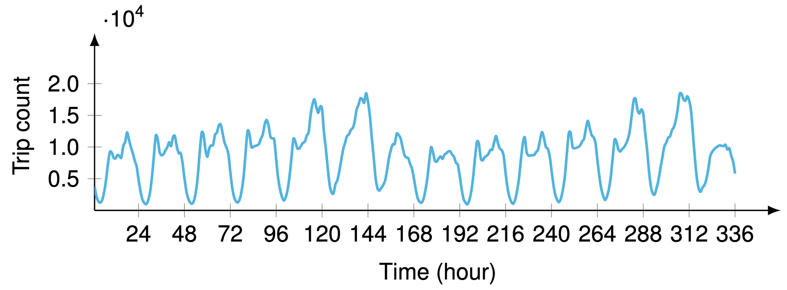
Figure 1. Hourly time series of aggregated ridesharing trip counts in the City of Chicago during the first two weeks (i.e., $2\times 7\times 24=336$ hours in total) since April 1, 2024. The time series exhibits weekly periodicity, referring to the regularity of human mobility.
I-A. Definition of Autoregression
The essential idea of time series autoregression is that a given data point of a time series is linearly dependent on the previous data points. Mathematically, the $d$th-order univariate autoregression of time series $\boldsymbol{x}=(x_1,x_2,\cdots,x_{T})^\top\in\mathbb{R}^{T}$ can be written as follows,
\[x_{t}=\sum_{k=1}^{d}w_{k}x_{t-k}+\epsilon_{t} \tag{1}\]for all \(t\in\{d+1,d+2,\ldots,T\}\). The integer $d\in\mathbb{Z}^{+}$ is the order. Here, $x_{t}\in\mathbb{R}$ is the value of the time series at time $t$. The vector $\boldsymbol{w}=(w_1,w_2,\cdots,w_{d})^\top\in\mathbb{R}^{d}$ represents the autoregressive coefficients. The random error $\epsilon_t\in\mathbb{R},\,\forall t$ is assumed to be normally distributed, following a mean of zero and a constant variance.
There is a closed-form solution to the coefficient vector $\boldsymbol{w}=(w_1,w_2,\cdots,w_{d})^\top\in\mathbb{R}^{d}$ from the optimization problem such that
\[\boldsymbol{w}:=\arg\,\min_{\boldsymbol{w}}\,\sum_{t=d+1}^{T}\Bigl(x_{t}-\sum_{k=1}^{d}w_{k}x_{t-k}\Bigr)^2 \tag{2}\]which is equivalent to
\[\boldsymbol{w}:=\arg\,\min_{\boldsymbol{w}}\,\|\tilde{\boldsymbol{x}}-\boldsymbol{A}\boldsymbol{w}\|_2^2=\boldsymbol{A}^{\dagger}\tilde{\boldsymbol{x}} \tag{3}\]where \(\|\cdot\|_2\) denotes the \(\ell_2\)-norm. The symbol \(\cdot^{\dagger}\) is the the Moore–Penrose inverse of a matrix. While using \(\ell_2\)-norm, the vector \(\tilde{\boldsymbol{x}}\) consists of the last \(T-d\) entries in the time series vector \(\boldsymbol{x}\), i.e.,
\[\tilde{\boldsymbol{x}}=\begin{bmatrix} x_{d+1} \\ x_{d+2} \\ \vdots \\ x_{T} \end{bmatrix}\in\mathbb{R}^{T-d}\]The matrix \(\boldsymbol{A}\) is also comprised of the entries in the time series vector \(\boldsymbol{x}\), which is given by
\[\boldsymbol{A}=\begin{bmatrix} x_{d} & x_{d-1} & \cdots & x_1 \\ x_{d+1} & x_{d} & \cdots & x_{2} \\ \vdots & \vdots & \ddots & \vdots \\ x_{T-1} & x_{T-2} & \cdots & x_{T-d} \end{bmatrix}\in\mathbb{R}^{(T-d)\times d}\]In essence, given the data pair \(\{\boldsymbol{A},\tilde{\boldsymbol{x}}\}\) constructed by the time series \(\boldsymbol{x}\), the univariate autoregression can be easily converted into a linear regression formula. Thus, the closed-form solution is least squares.
Considering one quick example:
I-B. Motivation of Sparse Autoregression
However, the challenges arise if there is a sparsity constraint in the form of \(\ell_0\)-norm, for instance,
\[\begin{aligned}\min_{\boldsymbol{w}}\,&\|\tilde{\boldsymbol{x}}-\boldsymbol{A}\boldsymbol{w}\|_2^2 \\ \text{s.t.}\,&\|\boldsymbol{w}\|_0\leq\tau \end{aligned}\]where the upper bound the constraint is an integer \(\tau\in\mathbb{Z}^{+}\), which is supposed to be no greater than the order \(d\). In the constraint, \(\|\boldsymbol{w}\|_0\) counts the number of nonzero entries in the vector \(\boldsymbol{w}\), and \(\tau\) is the sparsity level.
II. Sparse Autoregression
II-A. Mixed-Integer Programming
II-B. Semidefinite Programming
III. Time-Varying Sparse Autoregression
The optimization problem is formulated as follows,
\[\begin{aligned}\min_{\boldsymbol{w}_1,\boldsymbol{w}_{2},\ldots,\boldsymbol{w}_{\delta},\boldsymbol{\beta}}\,&\sum_{\gamma=1}^{\delta}\|\tilde{\boldsymbol{x}}_{\gamma}-\boldsymbol{A}_{\gamma}\boldsymbol{w}_{\gamma}\|_2^2 \\ \text{s.t.}\,&\begin{cases} \boldsymbol{\beta}\in\{0,1\}^{d} \\ -\alpha\cdot\boldsymbol{\beta}\leq \boldsymbol{w}_{\gamma}\leq\alpha\cdot\boldsymbol{\beta},\,\forall \gamma\in\{1,2,\ldots,\delta\} \\ \displaystyle \sum_{k=1}^{d}\beta_{k}=\|\boldsymbol{\beta}\|_1\leq\tau \end{cases} \end{aligned}\]Example 1. For any vectors \(\boldsymbol{x},\boldsymbol{y}\in\mathbb{R}^{n}\), verify that \(\boldsymbol{x}^\top\boldsymbol{y}=\operatorname{tr}(\boldsymbol{y}\boldsymbol{x}^\top)\).
According to the definition of inner product, we have \(\boldsymbol{x}^\top\boldsymbol{y}=\sum_{i=1}^{n}x_iy_i\). In contrast, the outer product between \(\boldsymbol{y}\) and \(\boldsymbol{x}\) is given by
\[\color{gray}\boldsymbol{y}\boldsymbol{x}^\top=\begin{bmatrix} y_1x_1 & y_1x_2 & \cdots & y_1x_n \\ y_2x_1 & y_2x_2 & \cdots & y_nx_2 \\ \vdots & \vdots & \ddots & \vdots \\ y_nx_1 & y_nx_2 & \cdots & y_nx_n \\ \end{bmatrix}\in\mathbb{R}^{n\times n}\]Recall that the trace of a square matrix is the sum of diagonal entries, we therefore have
\[\color{gray}\operatorname{tr}(\boldsymbol{y}\boldsymbol{x}^\top)=\sum_{i=1}^{n}y_ix_i=\boldsymbol{y}^\top\boldsymbol{x}=\boldsymbol{x}^\top\boldsymbol{y}\]as claimed.
III-A. Ridesharing Data
III-B. Formulating Time-Varying Systems
III-C. Solving the Optimization Problem
IV. Periodicity of Hangzhou Metro Passenger Flow
IV-A. Data Description
IV-B. Periodicity Analysis
IV-C. Spatially-Varying Systems
V. Wikipedia Traffic Time Series
Dataset
Wikipedia traffic time series dataset (see 145k dataset of daily Wikipedia traffic).
(Posted by Xinyu Chen on February 15, 2025)