Time Series Convolution
Convolutional kernel approaches for understanding the importance of time series trends and interpreting temporal patterns, allowing one to improve the performance of time series imputation and learn sparse representations of temporal correlations. In the imputation model, fast Fourier transform accelerates the optimization process with log-linear time complexity. In the interpretable machine learning, sparse regression unlocks opportunities to better capture the long-term changes and temporal patterns of real-world time series.
(Updated on March 31, 2025)
🔨 Annotating the weekly periodicity of hourly ridesharing trip time series in Chicago since April 1, 2024.
In this post, we intend to explain the essential ideas of our research work:
- Xinyu Chen, Zhanhong Cheng, HanQin Cai, Nicolas Saunier, Lijun Sun (2024). Laplacian convolutional representation for traffic time series imputation. IEEE Transactions on Knowledge and Data Engineering. 36 (11): 6490-6502.
- Xinyu Chen, Xi-Le Zhao, Chun Cheng (2024). Forecasting urban traffic states with sparse data using Hankel temporal matrix factorization. INFORMS Journal on Computing. Early access.
- Xinyu Chen, HanQin Cai, Fuqiang Liu, Jinhua Zhao (2025). Correlating time series with interpretable convolutional kernels. IEEE Transactions on Knowledge and Data Engineering. 37 (6): 3272-3283.
Content:
In Part I of this series, we introduce motivations of time series modeling with global and local trends. This is because global and local time series trends are important for improving the performance of time series imputation. Despite of this, we were always trying to formulate an appropriate interpretable machine learning model for quantifying the periodicity of time series. To clarify the modeling ideas, we identify some techincal stuff and elaborate on several key concepts such as circular convolution, convolution matrix, circulant matrix, and discrete Fourier transform in Part II.
Part III and Part IV give the modeling ideas of circulant matrix nuclear norm minimization and Laplacian convolutional representation, addressing the critical challenges in time series imputation tasks. The optimization algorithm of both models makes use of fast Fourier transform in a log-linear time complexity. Part V presents an interpretable convolutional kernel method in which the sparsity of convolutional kernels is modeled by $\ell_0$-norm induced sparsity constraints.
For an empirical evaluation, we demonstrate the interpretable convolutional kernels on ridesharing trip time series (see Part VI) and fluid flow data (see Part VII). These convolutional kernels allow one to quantify periodicity and seasonality underlying these dynamical system. Finally, Part VIII concludes the whole post.
I. Motivation
The development of machine learning models in the past decade has been truly remarkable. Convolution is one of the most commonly-used operations in the fields of applied mathematics and signal processing, which has been widely applied to several machine learning problems. The aims of this post are revisiting the essential ideas of circular convolution and laying an insightful foundation for modeling time series data.
Nowadays, although we have quite a lot of machine learning algorithms on hand, it is still necessary to rethink about the following perspectives in time series modeling:
- How to characterize global time series trends?
- How to characterize local time series trends?
- How to learn interpretable local and nonlocal patterns as convolutional kernels?
Sometimes, time series exhibit complicated trends if they are not stationary.
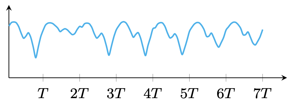
(a) Global trends (e.g., long-term daily/weekly periodicity)
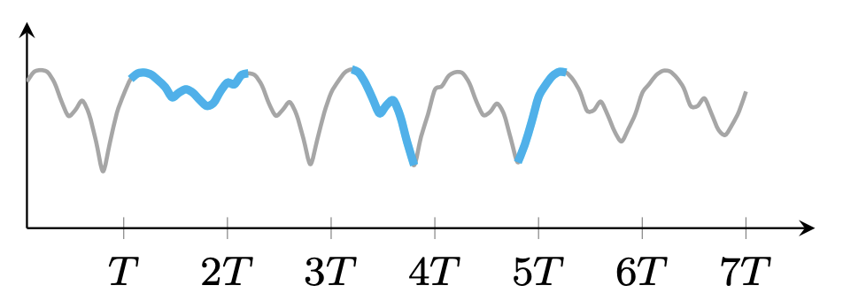
(b) Local trends (e.g., short-term time series trends)
Figure 1. Illustration of time series trends.
II. Preliminaries
In this study, we build the modeling concepts of Laplacian convolutional representation (LCR) upon several key essential ideas, including circular convolution, discrete Fourier transform, and fast Fourier transform, from the field of signal processing. In the following sections, we will discuss:
- What are circular convolution, convolution matrix, and circulant matrix?
- What is the convolution theorem?
- How can fast Fourier transform be used to compute the circular convolution?
- How do circular convolution and fast Fourier transform apply to Hankel matrix factorization?
II-A. Circular Convolution
Convolution is one of the most powerful operations in several deep learning frameworks, such as convolutional neural networks (CNNs). In the context of discrete sequences (typically vectors), circular convolution refers to the convolution of two discrete sequences of data, and it plays an important role in maximizing the efficiency of certain common filtering operations (see circular convolution on Wikipedia).
By definition, for any vectors $\boldsymbol{x}=(x_1,x_2,\cdots,x_T)^\top\in\mathbb{R}^{T}$ and $\boldsymbol{y}=(y_1,y_2,\cdots,y_\tau)^\top\in\mathbb{R}^{\tau}$ with $\tau\leq T$, the circular convolution (denoted by the “star” symbol $\star$) of these two vectors is formulated as follows,
\[\boldsymbol{z}=\boldsymbol{x}\star\boldsymbol{y}\in\mathbb{R}^{T} \tag{1}\]Elment-wise, we have the formula to specify a circular convolution operation:
\[z_{t}=\sum_{k=1}^{\tau}x_{t-k+1} y_{k},\,\forall t\in\{1,2,\ldots,T\} \tag{2}\]where $z_t$ represents the $t$th entry of $\boldsymbol{z}$. For a cyclical operation, it takes $x_{t-k+1}=x_{t-k+1+T}$ when $t+1\leq k$. While the definition of circular convolution might seem to be over-complicated for beginners, it becomes much easier when you consider the concept of a convolution or circulant matrix, as demonstrated in the examples provided below.
As mentioned above, the vector $\boldsymbol{x}$ has a length of $T$, and the vector $\boldsymbol{y}$ has a length of $\tau$. According to the definition of circular convolution, the resulting vector $\boldsymbol{z}$ will also have a length of $T$, matching the length of the original vector $\boldsymbol{x}$.
Given any vectors $\boldsymbol{x}=(x_1,x_2,x_3,x_4)^\top\in\mathbb{R}^4$ and $\boldsymbol{y}=(y_1,y_2,y_3)^\top\in\mathbb{R}^3$, the circular convolution between them can be expressed as follows,
\[\begin{aligned} \boldsymbol{z}=&\boldsymbol{x}\star\boldsymbol{y}=\begin{bmatrix} \displaystyle\sum_{k=1}^{3}x_{1-k+1}y_k \\ \displaystyle\sum_{k=1}^{3}x_{2-k+1}y_k \\ \displaystyle\sum_{k=1}^{3}x_{3-k+1}y_k \\ \displaystyle\sum_{k=1}^{3}x_{4-k+1}y_k \\ \end{bmatrix}=\begin{bmatrix} x_1y_1+x_0y_2+x_{-1}y_3 \\ x_2y_1+x_1y_2+x_{0}y_3 \\ x_3y_1+x_2y_2+x_1y_3 \\ x_4y_1+x_3y_2+x_2y_3 \\ \end{bmatrix} \\ \Rightarrow\boldsymbol{z}=&\begin{bmatrix} x_1y_1+x_4y_2+x_3y_3 \\ x_2y_1+x_1y_2+x_4y_3 \\ x_3y_1+x_2y_2+x_1y_3 \\ x_4y_1+x_3y_2+x_2y_3 \\ \end{bmatrix} \\ \end{aligned}\]where $x_{0}=x_4$ and $x_{-1}=x_3$ according to the definition.
In this case, each entry $z_t$ of the resulting vector $\boldsymbol{z}$ is computed as the inner product between the vector $\boldsymbol{y}$ and a reversed and truncated version of the vector $\boldsymbol{x}$. Specifically, the entry $z_1$ is obtained by computing the inner product between $(x_1,x_4,x_3)^\top$ and $(y_1,y_2,y_3)^\top$, or check out the following one:
\[z_1=\begin{bmatrix} x_1 & x_4 & x_3 \end{bmatrix} \begin{bmatrix} y_1 \\ y_2 \\ y_3 \end{bmatrix}=x_1y_1+x_4y_2+x_3y_3\]For subsequent entries $z_2,z_3,z_4$, the vector $\boldsymbol{x}$ is cyclically shifted in reverse and truncated (only preserving the first $\tau$ entries), and then the inner product with $\boldsymbol{y}$ is calculated. Figure 2 illustrates the basic steps for computing each entry of the circular convolution.
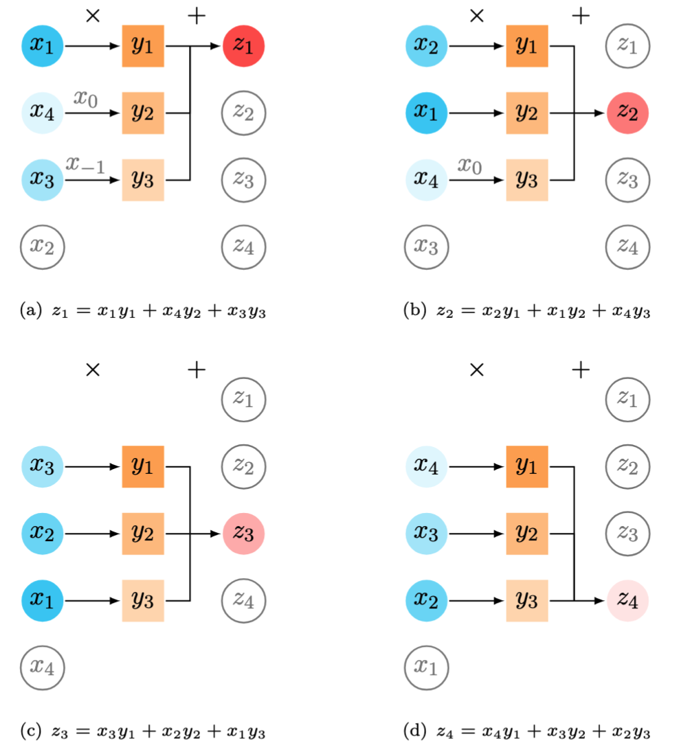
Figure 2. Illustration of the circular convolution between $\boldsymbol{x}=(x_1,x_2,x_3,x_4)^\top$ and $\boldsymbol{y}=(y_1,y_2,y_3)^\top$. (a) Computing $z_1$ involves $x_{0}=x_4$ and $x_{-1}=x_3$. (b) Computing $z_2$ involves $x_{0}=x_4$. The figure is inspired by Prince (2023) and But what is convolution? (created by 3blue1brown).
As can be seen, circular convolution between two vectors can essentially be viewed as a linear operation. This perspective allows one to reformulate the circular convolution as a linear transformation using a convolution matrix. In the case of two vectors of the same length, the linear transformation is written with a circulant matrix.
Example 1. Given vectors $\boldsymbol{x}=(0,1,2,3,4)^\top$ and $\boldsymbol{y}=(2,-1,3)^\top$, the circular convolution $\boldsymbol{z}=\boldsymbol{x}\star\boldsymbol{y}=(5,14,3,7,11)^\top$ has the following entries:
\[\color{gray}\begin{cases} z_1=x_1y_1+x_5y_2+x_4y_3=0\times 2+4\times(-1)+3\times 3=5 \\ z_2=x_2y_1+x_1y_2+x_5y_3=1\times 2+0\times(-1)+4\times 3=14 \\ z_3=x_3y_1+x_2y_2+x_1y_3=2\times 2+1\times (-1)+0\times 3=3 \\ z_4=x_4y_1+x_3y_2+x_2y_3=3\times 2+2\times (-1)+1\times 3=7 \\ z_5=x_5y_1+x_4y_2+x_3y_3=4\times 2+3\times (-1)+2\times 3=11 \end{cases}\]where $x_{0}=x_5$ and $x_{-1}=x_4$ according to the definition.
II-B. Convolution Matrix
Using the notations above, for any vectors $\boldsymbol{x}\in\mathbb{R}^{T}$ and $\boldsymbol{y}\in\mathbb{R}^{\tau}$ with $\tau<T$, the circular convolution can be expressed as a linear transformation:
\[\boldsymbol{z}=\boldsymbol{x}\star\boldsymbol{y}=\mathcal{C}_{\tau}(\boldsymbol{x})\boldsymbol{y} \tag{3}\]where $\mathcal{C}_{\tau}:\mathbb{R}^{T}\to\mathbb{R}^{T\times \tau}$ denotes the convolution operator with the hyperparameter $\tau$ (positive integer). The convolution matrix can be represented as follows,
\[\mathcal{C}_{\tau}(\boldsymbol{x})=\begin{bmatrix} x_1 & x_T & x_{T-1} & \cdots & x_{T-\tau+2} \\ x_2 & x_1 & x_{T} & \cdots & x_{T-\tau+3} \\ x_3 & x_2 & x_1 & \cdots & x_{T-\tau+4} \\ \vdots & \vdots & \vdots & \ddots & \vdots \\ x_{T} & x_{T-1} & x_{T-2} & \cdots & x_{T-\tau+1} \\ \end{bmatrix}\in\mathbb{R}^{T\times\tau}\]In the feild of signal processing, this linear transformation is one of the most fundamental properties of circular convolution, highlighting its role in efficently implementing filtering operations.
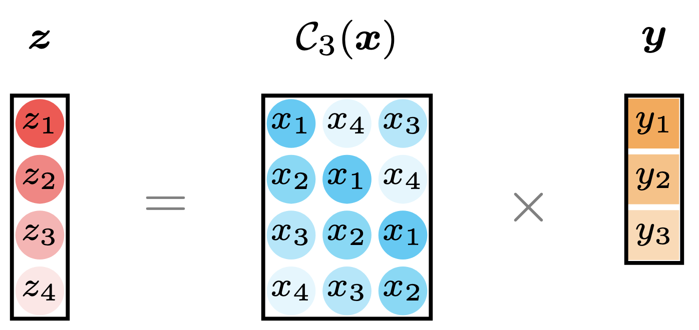
Figure 3. Illustration of circular convolution as the linear transformation with a convolution matrix.
Example 2. Given vectors $\boldsymbol{x}=(0,1,2,3,4)^\top$ and $\boldsymbol{y}=(2,-1,3)^\top$, the circular convolution $\boldsymbol{z}=\boldsymbol{x}\star\boldsymbol{y}$ can be expressed as:
\[\color{gray}\boldsymbol{z}=\boldsymbol{x}\star\boldsymbol{y}=\mathcal{C}_{3}(\boldsymbol{x})\boldsymbol{y}\]where $\mathcal{C}_{3}(\boldsymbol{x})$ is the convolution matrix with $\tau=3$ columns. Specifically, the convolution matrix is given by
\[\color{gray}\mathcal{C}_{3}(\boldsymbol{x})=\begin{bmatrix} 0 & 4 & 3 \\ 1 & 0 & 4 \\ 2 & 1 & 0 \\ 3 & 2 & 1 \\ 4 & 3 & 2 \end{bmatrix}\]As a result, it gives
\[\color{gray}\boldsymbol{z}=\mathcal{C}_{3}(\boldsymbol{x})\boldsymbol{y}=\begin{bmatrix} 0 & 4 & 3 \\ 1 & 0 & 4 \\ 2 & 1 & 0 \\ 3 & 2 & 1 \\ 4 & 3 & 2 \end{bmatrix}\begin{bmatrix} 2 \\ -1 \\ 3 \end{bmatrix}=\begin{bmatrix} 5 \\ 14 \\ 3 \\ 7 \\ 11 \end{bmatrix}\]This representation shows that circular convolution is equivalent to a matrix-vector multiplication, making it easier to understand, especially in signal processing applications.
In this post, we aim to make the concepts clear and accessible by incorporting programming code in Python, intuitive illustrations, and detailed explanations of the formulas. To demonstrate how circular convolution can be computed, we use Python’s numpy library. First, we construct the convolution matrix on the vector $\boldsymbol{x}$ and then perform the circular convolution as follows.
import numpy as np

def conv_mat(vec, tau):
    n = vec.shape[0]
    mat = np.zeros((n, tau))
    mat[:, 0] = vec
    for i in range(1, tau):
        mat[:, i] = np.append(vec[-i :], vec[: n - i], axis = 0)
    return mat

x = np.array([0, 1, 2, 3, 4])
y = np.array([2, -1, 3])
mat = conv_mat(x, y.shape[0])
print('Convolution matrix of x with 3 columns:')
print(mat)
print()
z = mat @ y
print('Circular convolution of x and y:')
print(z)
II-C. Circulant Matrix
Recall that the convolution matrix $\mathcal{C}_{\tau}(\boldsymbol{x})$ is specified with $\tau$ columns, corresponding to the length of vector $\boldsymbol{y}$). In the case of $\boldsymbol{x},\boldsymbol{y}\in\mathbb{R}^{T}$ with same columns, the convolution matrix becoms a square matrix, known as a circulant matrix. In this study, we emphasize the importance of circulant matrices and their properties, such as their strong connection with circular convolution and discrete Fourier transform, even through we do not work directly with circulant matrices.
For any vectors $\boldsymbol{x},\boldsymbol{y}\in\mathbb{R}^{T}$, the circular convolution can be expressed as a linear transformation such that
\[\boldsymbol{z}=\boldsymbol{x}\star\boldsymbol{y}=\mathcal{C}(\boldsymbol{x})\boldsymbol{y} \tag{4}\]where $\mathcal{C}:\mathbb{R}^{T}\to\mathbb{R}^{T\times T}$ denotes the circulant operator. The circulant matrix is defined as:
\[\mathcal{C}(\boldsymbol{x})=\begin{bmatrix} x_1 & x_T & x_{T-1} & \cdots & x_{2} \\ x_2 & x_1 & x_{T} & \cdots & x_{3} \\ x_3 & x_2 & x_1 & \cdots & x_{4} \\ \vdots & \vdots & \vdots & \ddots & \vdots \\ x_{T} & x_{T-1} & x_{T-2} & \cdots & x_{1} \\ \end{bmatrix}\in\mathbb{R}^{T\times T}\]which forms a square matrix. It always holds that $|\mathcal{C}(\boldsymbol{x})|_F=\sqrt{T}\cdot|\boldsymbol{x}|_2$ where $|\cdot|_F$ and $|\cdot|_2$ are the Frobenius norm of matrix and the $\ell_2$-norm of vector, respectively.
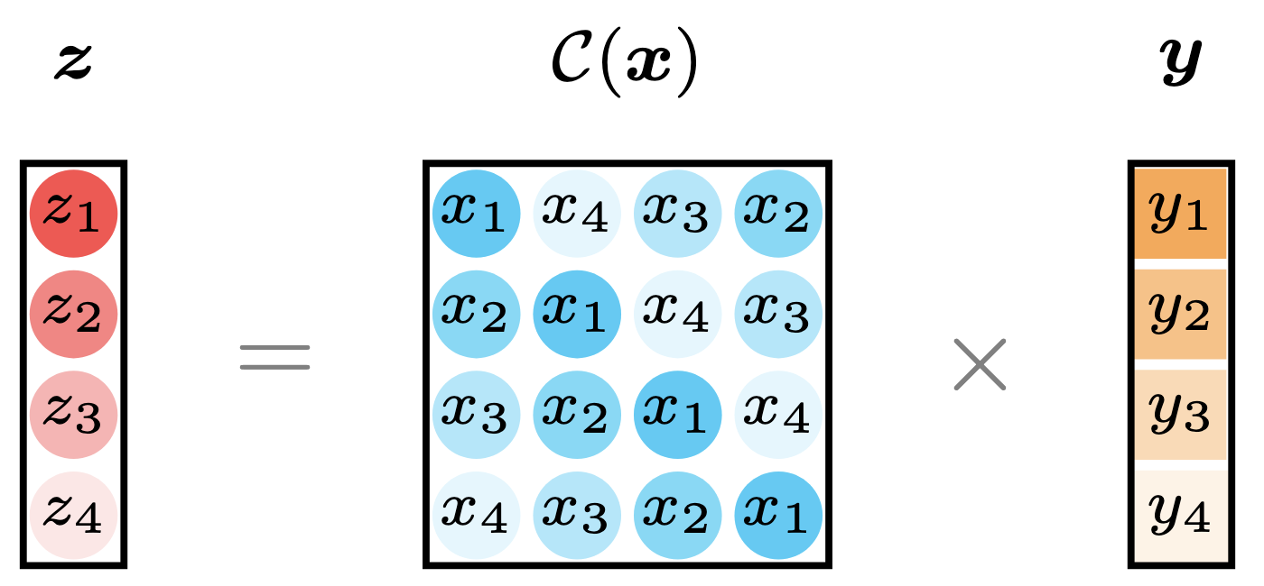
Figure 4. Illustration of circular convolution as the linear transformation with a circulant matrix.
Example 3. Given vectors $\boldsymbol{x}=(0,1,2,3,4)^\top$ and $\boldsymbol{y}=(2,-1,3,0,0)^\top$, the circular convolution $\boldsymbol{z}=\boldsymbol{x}\star\boldsymbol{y}$ is identical to
\[\color{gray}\boldsymbol{z}=\boldsymbol{x}\star\boldsymbol{y}=\mathcal{C}(\boldsymbol{x})\boldsymbol{y}=(5,14,3,7,11)^\top\]where $\mathcal{C}(\boldsymbol{x})$ is the circulant matrix formed from $\boldsymbol{x}$ such that
\[\color{gray}\mathcal{C}(\boldsymbol{x})=\begin{bmatrix} 0 & 4 & 3 & 2 & 1 \\ 1 & 0 & 4 & 3 & 2 \\ 2 & 1 & 0 & 4 & 3 \\ 3 & 2 & 1 & 0 & 4 \\ 4 & 3 & 2 & 1 & 0 \end{bmatrix}\]Thus, the result can be written as follows,
\[\color{gray}\boldsymbol{z}=\mathcal{C}(\boldsymbol{x})\boldsymbol{y}=\begin{bmatrix} 0 & 4 & 3 & 2 & 1 \\ 1 & 0 & 4 & 3 & 2 \\ 2 & 1 & 0 & 4 & 3 \\ 3 & 2 & 1 & 0 & 4 \\ 4 & 3 & 2 & 1 & 0 \end{bmatrix}\begin{bmatrix} 2 \\ -1 \\ 3 \\ 0 \\ 0 \end{bmatrix}=\begin{bmatrix} 5 \\ 14 \\ 3 \\ 7 \\ 11 \end{bmatrix}\]The example shows that the circular convolution of $\boldsymbol{x}$ and $(2,-1,3)^\top$ is equivalent to the circular convolution of $\boldsymbol{x}$ and $\boldsymbol{y}$ with its last two entries padded with zeros. Thus, to compute the circular convolution of $\boldsymbol{x}\in\mathbb{R}^{T}$ and $\boldsymbol{y}\in\mathbb{R}^{\tau}$ when $T$ is greater than $\tau$, one can simply append $T-\tau$ zeros to the end of $\boldsymbol{y}$ and perform the circular convolution.
II-D. Discrete Fourier Transform
Discrete Fourier transform (see Wikipedia) is a fundamental tool in mathematics and signal processing with widespread applications to machine learning. The discrete Fourier transform is the key discrete transform used for Fourier analysis, enabling the decomposition of a signal into its constituent frequencies. The fast Fourier transform is an efficient algorithm for computing the discrete Fourier tranform (see the difference between discrete Fourier transform and fast Fourier transform), significantly reducing the time complexity from $\mathcal{O}(T^2)$ to $\mathcal{O}(T\log T)$, where $T$ is the number of data points. This efficiency makes fast Fourier transform essential for processing large problems.
A crucial concept in signal processing is the convolution theorem, which states that convolution in the time domain is the multiplication in the frequency domain. This implies that the circular convolution can be efficiently computed by using the fast Fourier transform. The convolution theorem for discrete Fourier transform is summarized as follows,
\[\mathcal{F}(\boldsymbol{x}\star\boldsymbol{y})=\mathcal{F}(\boldsymbol{x})\circ\mathcal{F}(\boldsymbol{y}) \tag{5}\]or
\[\boldsymbol{x}\star\boldsymbol{y}=\mathcal{F}^{-1}(\mathcal{F}(\boldsymbol{x})\circ\mathcal{F}(\boldsymbol{y})) \tag{6}\]where $\mathcal{F}(\cdot)$ and $\mathcal{F}^{-1}(\cdot)$ denote the discrete Fourier transform and the inverse discrete Fourier transform, respectively. The symbol $\circ$ represents the Hadamard product, i.e., element-wise multiplication.
In fact, this principle underlies many efficient algorithms in signal processing and data analysis, allowing complex operations to be performed efficiently in the frequency domain.
Example 4. Given vectors $\boldsymbol{x}=(0,1,2,3,4)^\top$ and $\boldsymbol{y}=(2,-1,3,0,0)^\top$, the circular convolution $\boldsymbol{z}=\boldsymbol{x}\star\boldsymbol{y}$ can be computed via the use of fast Fourier transform in numpy as follows,
import numpy as np

x = np.array([0, 1, 2, 3, 4])
y = np.array([2, -1, 3, 0, 0])
fx = np.fft.fft(x)
fy = np.fft.fft(y)
z = np.fft.ifft(fx * fy).real
print('Fast Fourier transform of x:')
print(fx)
print('Fast Fourier transform of y:')
print(fy)
print('Circular convolution of x and y:')
print(z)
in which the outputs are
Fast Fourier transform of x:
[10. +0.j         -2.5+3.4409548j  -2.5+0.81229924j -2.5-0.81229924j
 -2.5-3.4409548j ]
Fast Fourier transform of y:
[ 4.        +0.j         -0.73606798-0.81229924j  3.73606798+3.4409548j
  3.73606798-3.4409548j  -0.73606798+0.81229924j]
Circular convolution of x and y:
[ 5. 14.  3.  7. 11.]
II-F. Hankel Matrix Factorization & Discrete Fourier Transform
Hankel matrix plays a fundamental role in numerous areas of applied mathematics and signal processing. By definition, a Hankel matrix is a square or rectangular matrix in which each ascending skew-diagonal (from left to right) has the same value. Given vector $\boldsymbol{x}\in\mathbb{R}^{T}$, the Hankel matrix can be constructed as follows,
\[\mathcal{H}(\boldsymbol{x})=\begin{bmatrix} x_1 & x_2 & \cdots & x_{T-n+1} \\ x_2 & x_3 & \cdots & x_{T-n+2} \\ \vdots & \vdots & \ddots & \vdots \\ x_{n} & x_{n+1} & \cdots & x_{T} \end{bmatrix}\]where the Hankel matrix has $n$ rows and $T-n+1$ columns. This matrix is often used to represent signals or time series data, capturing their sequential dependencies and structure, see e.g., Chen et al. (2024) in our work.
On the Hankel matrix $\mathcal{H}(\boldsymbol{x})$, if it can be approximated by the multiplication of two matrices $\boldsymbol{W}\in\mathbb{R}^{n\times R}$ and $\boldsymbol{Q}\in\mathbb{R}^{(T-n+1)\times R}$, then one can compute the inverse of Hankel matrix factorization as follows,
\[\begin{aligned} \mathcal{H}(\boldsymbol{x})\approx&\boldsymbol{W}\boldsymbol{Q}^\top \\ \Rightarrow\quad\tilde{\boldsymbol{x}}=&\mathcal{H}^{\dagger}(\boldsymbol{W}\boldsymbol{Q}^{\top}) \\ \Rightarrow\quad\tilde{x}_t=&\frac{1}{\rho_t}\sum_{a+b=t+1}\boldsymbol{w}_{a}^\top\boldsymbol{q}_{b} \\ \Rightarrow\quad\tilde{x}_{t}=&\frac{1}{\rho_t}\sum_{r=1}^{R}\underbrace{\sum_{a+b=t+1}w_{a,r}q_{b,r}}_{\color{red}\text{circular convolution}} \end{aligned} \tag{7}\]where $\boldsymbol{w}_a$ and $\boldsymbol{q}_b$ are the $a$-th and $b$-th rows of $\boldsymbol{W}$ and $\boldsymbol{Q}$, respectively. Herein, $\mathcal{H}^{\dagger}(\cdot)$ denotes the inverse operator of Hankel matrix. For any matrix $\boldsymbol{Y}$ of size $n\times (T-n+1)$, the inverse operator is given by
\[[\mathcal{H}^{\dagger}(\boldsymbol{Y})]_{t}=\frac{1}{\rho_{t}}\sum_{a+b=t+1}y_{a,b} \tag{8}\]where $t\in{1,2,\cdots, T}$. $\rho_t$ is the number of entries on the $t$-th antidiagonal of the $n\times (T-n+1)$ matrix, satisfying
\[\rho_t=\begin{cases} t, & t\leq\min\{n, T-n+1\} \\ T-t+1, & \text{otherwise} \end{cases} \tag{9}\]Following the aforementioned formula, it is easy to connect the Hankel factorization with circular convolution and discrete Fourier transform (Cai et al., 2019; Cai et al., 2022) such that
\[\tilde{x}_{t}=\frac{1}{\rho_t}\sum_{r=1}^{R}[\tilde{\boldsymbol{w}}_r\star\tilde{\boldsymbol{q}}_r]_{t}=\frac{1}{\rho_t}\sum_{r=1}^{R}[\mathcal{F}^{-1}(\mathcal{F}(\tilde{\boldsymbol{w}}_r)\circ\mathcal{F}(\tilde{\boldsymbol{q}}_r))]_{t} \tag{10}\]where we define two vectors:
\[\begin{cases} \tilde{\boldsymbol{w}}_{r}=(w_{1,r},w_{2,r},\cdots,w_{t,r})^\top \\ \tilde{\boldsymbol{q}}_{r}=(q_{1,r},q_{2,r},\cdots,q_{t,r})^\top \end{cases}\]of length $t$. The notation $[\cdot]_{t}$ refers to the $t$th entry of the vector. Notably, they are different from the vectors $\boldsymbol{w}_r\in\mathbb{R}^{n}$ and $\boldsymbol{q}_r\in\mathbb{R}^{T-n+1}$. If $t\leq n$, then the vector $\tilde{\boldsymbol{w}}_r$ consists of the first $t$ entries of $\boldsymbol{w}_r$. If $t> n$, then the vector $\tilde{\boldsymbol{w}}_r$ consists of the vector $\boldsymbol{w}_r$ and $t-n$ zeros, i.e.,
\[\tilde{\boldsymbol{w}}_r=(w_{1,r},w_{2,r},\cdots,w_{n,r},\underbrace{0,\cdots,0}_{t-n})^\top\in\mathbb{R}^{t}\]This principle is well-suited to the construction of vector $\tilde{\boldsymbol{q}}_r$. In order to compute each $\tilde{x}_t,\forall t\in{1,2,\ldots,n}$, the time complexity of the aforementioned circular convolution is $\mathcal{O}(R\cdot t\log t)$, and the element-wise multiplication takes $\mathcal{C}(R\cdot t)$.
Example 5. Given vector $\boldsymbol{x}=(x_1,x_2,\cdots,x_6)^\top\in\mathbb{R}^{6}$, let the number of rows of the Hankel matrix be $4$, the Hankel matrix is given by
\[\color{gray}\mathcal{H}(\boldsymbol{x})=\begin{bmatrix} x_1 & x_2 & x_3 \\ x_2 & x_3 & x_4 \\ x_3 & x_4 & x_5 \\ x_4 & x_5 & x_6 \end{bmatrix}\]If it takes a rank-one approximation such that $\mathcal{H}(\boldsymbol{x})\approx\boldsymbol{w}\boldsymbol{q}^\top$ with $\boldsymbol{w}\in\mathbb{R}^{4}$ and $\boldsymbol{q}\in\mathbb{R}^{3}$, then the inverse of Hankel matrix factorization can be written as follows,
\[\color{gray}\begin{aligned} \tilde{x}_1&=\frac{1}{1}\sum_{a+b=2}w_aq_b=w_1q_1 \\ \tilde{x}_2&=\frac{1}{2}\sum_{a+b=3}w_aq_b=\frac{1}{2}(w_1q_2+w_2q_1) \\ &=\frac{1}{2}[(w_1,w_2)\star(q_1,q_2)]_{2} \\ \tilde{x}_3&=\frac{1}{3}\sum_{a+b=4}w_aq_b=\frac{1}{3}(w_1q_3+w_2q_2+w_3q_1) \\ &=\frac{1}{3}[(w_1,w_2,w_3)\star(q_1,q_2,q_3)]_{3} \\ \tilde{x}_4&=\frac{1}{3}\sum_{a+b=5}w_aq_b=\frac{1}{3}(w_2q_3+w_3q_2+w_4q_1) \\ &=\frac{1}{3}[(w_1,w_2,w_3,w_4)\star(q_1,q_2,q_3,0)]_{4} \\ \tilde{x}_5&=\frac{1}{2}\sum_{a+b=6}w_aq_b=\frac{1}{2}(w_3q_3+w_4q_2) \\ &=\frac{1}{2}[(w_1,w_2,w_3,w_4,0)\star(q_1,q_2,q_3,0,0)]_{5} \\ \tilde{x}_6&=\frac{1}{1}\sum_{a+b=7}w_aq_b=w_4q_3 \\ &=[(w_1,w_2,w_3,w_4,0,0)\star(q_1,q_2,q_3,0,0,0)]_{6} \end{aligned}\]which can be converted into circular convolution. By doing so, the computing process can be implemented with fast Fourier transform.
Acknowledgement. Thank you @Jinming Yang for correcting the notational mistake of circular convolution in this example.
Example 5 verifies the connection between Hankel matrix and circular convolution. The principle of circular convolution can be seamlessly incorporated into the inverse of Hankel matrix factorization.
Time complexity. Given the Hankel matrix factorization formula as $\tilde{\boldsymbol{x}}=\mathcal{H}^{\dagger}(\boldsymbol{w}\boldsymbol{q}^\top)$ where $\boldsymbol{w}\in\mathbb{R}^{n}$ and $\boldsymbol{q}\in\mathbb{R}^{n}$, suppose $T=2n-1$, the number of operations for computing the vector $\tilde{\boldsymbol{x}}$ in the element-wise multiplication is
\[\color{gray}1+2+\cdots+n=\frac{n(n-1)}{2}\]leading to $\mathcal{O}(n^2)$ time complexity. Following the inverse of Hankel matrix factorization in Example 5, the number of operations is
\[\color{gray}2(1+2+\cdots+\operatorname{floor}(\frac{n}{2}))=\operatorname{floor}(\frac{n}{2})(1+\operatorname{floor}(\frac{n}{2}))\]if $n$ is odd. Otherwise, the number of operations is
\[\color{gray}2(1+2+\cdots+\frac{n}{2})-\frac{n}{2}=\frac{n}{2}(1+\frac{n}{2})-\frac{n}{2}\]Figure 5 shows the empirical time complexity of the inverse of Hankel matrix factorization with element-wise multiplication and circular convolution, respectively. If one uses circular convolution with fast Fourier transform, then the computational cost of inverse operations is about 100 fold compared to the element-wise multiplication. It turns out that the element-wise multiplication is more efficient than the circular convolution in this case.
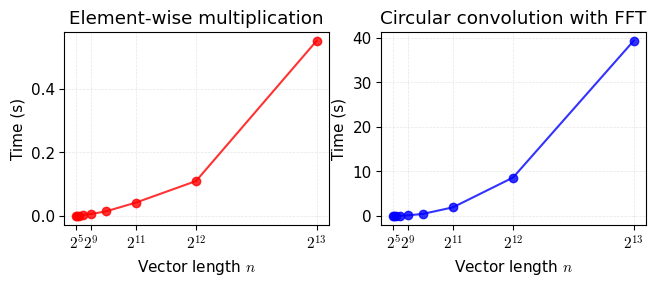
Figure 5. Empirical time complexity of the inverse of Hankel matrix factorization $\tilde{\boldsymbol{x}}=\mathcal{H}^{\dagger}(\boldsymbol{w}\boldsymbol{q}^\top)$ where $\boldsymbol{w}\in\mathbb{R}^{n}$ and $\boldsymbol{q}\in\mathbb{R}^{T-n+1}$. Note that we set the vector length as $n\in{2^5,2^6,\ldots,2^{13}}$ and $T=2n-1$. We repeat the numerical experiments 100 times corresponding to each vector length.
import numpy as np

def inverse_hankel(w, q, fft = False):
    dim1 = w.shape[0]
    dim2 = q.shape[0]
    dim = min(dim1, dim2)
    T = dim1 + dim2 - 1
    x_tilde = np.zeros(T)
    for t in range(T):
        w_new = np.zeros(t + 1)
        if t < dim1:
            w_new[: t + 1] = w[: t + 1]
        elif t >= dim1:
            w_new[: dim1] = w
        q_new = np.zeros(t + 1)
        if t < dim2:
            q_new[: t + 1] = q[: t + 1]
        elif t >= dim2:
            q_new[: dim2] = q
        if t < dim:
            rho = t + 1
        else:
            rho = T - (t + 1) + 1
        if fft == True:
            vec = np.fft.ifft(np.fft.fft(w_new) * np.fft.fft(q_new)).real
            x_tilde[t] = vec[t] / rho
        elif fft == False:
            x_tilde[t] = np.inner(w_new, np.flip(q_new)) / rho
    return x_tilde
For the entire implementation, please check out Appendix.
Example 6. For any vector $\boldsymbol{x}\in\mathbb{R}^{T}$, it always holds that
\[\color{gray}\|\mathcal{H}(\mathcal{D}(\boldsymbol{x}))\|_F=\|\boldsymbol{x}\|_2\]in which the operator $\mathcal{D}(\cdot)$ is defined as follows,
\[\color{gray}\mathcal{D}(\boldsymbol{x})=\bigr(x_1,\frac{1}{\sqrt{\rho_2}}x_2,\frac{1}{\sqrt{\rho_3}}x_3,\cdots,\frac{1}{\sqrt{\rho_{T-1}}}x_{T-1},x_T\bigl)^\top\in\mathbb{R}^{T}\]Verify this property on the vector $\boldsymbol{x}=(x_1,x_2,\cdots,x_6)^\top$ if the number of rows of the Hankel matrix is set as $4$.
According to the defintion, we have
\[\color{gray}\mathcal{D}(\boldsymbol{x})=\bigr(x_1,\frac{1}{\sqrt{2}}x_2,\frac{1}{\sqrt{3}}x_3,\frac{1}{\sqrt{3}}x_4,\frac{1}{\sqrt{2}}x_{5},x_6\bigl)^\top\]The Hankel matrix is given by
\[\color{gray}\mathcal{H}(\mathcal{D}(\boldsymbol{x}))=\begin{bmatrix} x_1 & \frac{1}{\sqrt{2}}x_2 & \frac{1}{\sqrt{3}}x_3 \\ \frac{1}{\sqrt{2}}x_2 & \frac{1}{\sqrt{3}}x_3 & \frac{1}{\sqrt{3}}x_4 \\ \frac{1}{\sqrt{3}}x_3 & \frac{1}{\sqrt{3}}x_4 & \frac{1}{\sqrt{2}}x_5 \\ \frac{1}{\sqrt{3}}x_4 & \frac{1}{\sqrt{2}}x_5 & x_6 \end{bmatrix}\]Thus, the Frobenius norm of this Hankel matrix is equivalent to the $\ell_2$-norm of the vector $\boldsymbol{x}$.
III. Circulant Matrix Nuclear Norm Minimization
Circulant matrix is commonly used to many computational and theoretical aspects of signal processing and machine learning, providing an efficient framework for implementating various algorithms such as circulant matrix nuclear norm minimization. By definition, a circulant matrix is a special square matrix where which shifts the previous row to the right by one position, with the last entry wrapping around to the first position. As we already discussed the circulant matrix above, we will present the circulant matrix nuclear norm, its optimization problem, and applications.
III-A. Definition
Nuclear norm is a key concept in matrix computations and convex optimization, frequently applied in low-rank matrix approximation and completion problems. For any matrix $\boldsymbol{X}\in\mathbb{R}^{m\times n}$, the nuclear norm is defined as the sum of singular values:
\[\left\|\boldsymbol{X}\right\|_{*}=\sum_{r=1}^{t}s_{r} \tag{11}\]where $\Vert\cdot\Vert_*$ denotes the nuclear norm. As illustrated in Figure 6, the singular values are $s_1,s_2,\ldots, s_t$ with $t=\min\lbrace m,n\rbrace$.
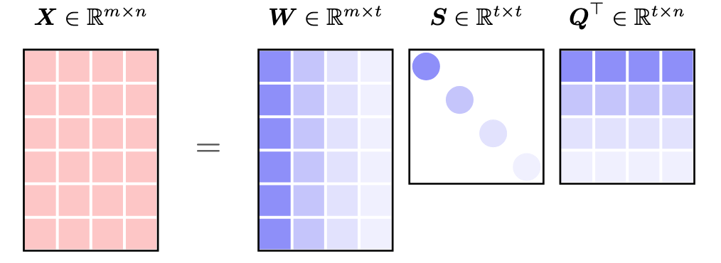
Figure 6. Singular value decomposition of matrix $\boldsymbol{X}\in\mathbb{R}^{m\times n}$. In the decomposed matrices, the unitary matrix $\boldsymbol{W}\in\mathbb{R}^{m\times t}$ (or $\boldsymbol{Q}\in\mathbb{R}^{n\times t}$) consists of $t$ orthogonal left (or right) singular vectors, while the $t$ diagonal entries of $\boldsymbol{S}$ are singular values such that $s_1\geq s_2\geq\cdots\geq s_t\geq 0$.
Example 7. Given vector $\boldsymbol{x}=(0,1,2,3,4)^\top$, the circulant matrix is
\[\color{gray}\mathcal{C}(\boldsymbol{x})=\begin{bmatrix} 0 & 4 & 3 & 2 & 1 \\ 1 & 0 & 4 & 3 & 2 \\ 2 & 1 & 0 & 4 & 3 \\ 3 & 2 & 1 & 0 & 4 \\ 4 & 3 & 2 & 1 & 0 \end{bmatrix}\]Thus, the singular values are
\[\color{gray}\boldsymbol{s}=(10, 4.25325404, 4.25325404, 2.62865556, 2.62865556)^\top\]As a result, we have the nuclear norm as follows,
\[\color{gray}\left\|\mathcal{C}(\boldsymbol{x})\right\|_{*}=\sum_{t=1}^{5}s_t=23.7638\]
Please reproduce the results by using the following numpy implementation.
import numpy as np

def circ_mat(vec):
    n = vec.shape[0]
    mat = np.zeros((n, n))
    mat[:, 0] = vec
    for i in range(1, n):
        mat[:, i] = np.append(vec[-i :], vec[: n - i], axis = 0)
    return mat

x = np.array([0, 1, 2, 3, 4])
mat = circ_mat(x)
w, s, q = np.linalg.svd(mat, full_matrices = False)
print('Singular values of C(x):')
print(s)
III-B. Property
One of the most intriguing properties of circulant matrices is that they are diagonalizable by the discrete Fourier transform matrix. The eigenvalue decomposition of circulant matrix $\mathcal{C}(\boldsymbol{x})\in\mathbb{R}^{T\times T}$ (constructed from any vector $\boldsymbol{x}\in\mathbb{R}^T$) is given by
\[\mathcal{C}(\boldsymbol{x})=\boldsymbol{F}\operatorname{diag}(\mathcal{F}(\boldsymbol{x}))\boldsymbol{F}^H \tag{12}\]where $\boldsymbol{F}$ is the unitary discrete Fourier transform matrix, $\boldsymbol{F}^H$ is the Hermitian transpose of $\boldsymbol{F}$, and $\mathcal{F}(\boldsymbol{x})$ is a diagonal matrix containing the eigenvalues of $\mathcal{C}(\boldsymbol{x})$. Due to this property, the nuclear norm of the circulant matrix can be formulated as the $\ell_1$-norm of the discrete Fourier transform of the vector $\boldsymbol{x}$:
\[\begin{aligned} \|\mathcal{C}(\boldsymbol{x})\|_*=&\|\boldsymbol{F}\operatorname{diag}(\mathcal{F}(\boldsymbol{x}))\boldsymbol{F}^H\|_{*} \\ =&\|\operatorname{diag}(\mathcal{F}(\boldsymbol{x}))\|_* \\ =&\|\mathcal{F}(\boldsymbol{x})\|_1 \end{aligned} \tag{13}\]This relationship draws a strong connection between circulant matrices and Fourier analysis, enabling efficient computation and analysis in various applications, e.g., circulant matrix nuclear norm minimization (Chen et al., 2024).
Example 8. Given vector $\boldsymbol{x}=(0,1,2,3,4)^\top$, the circulant matrix is
\[\color{gray}\mathcal{C}(\boldsymbol{x})=\begin{bmatrix} 0 & 4 & 3 & 2 & 1 \\ 1 & 0 & 4 & 3 & 2 \\ 2 & 1 & 0 & 4 & 3 \\ 3 & 2 & 1 & 0 & 4 \\ 4 & 3 & 2 & 1 & 0 \end{bmatrix}\]
The eigenvalues of $\mathcal{C}(\boldsymbol{x})$ and the fast Fourier transform of $\boldsymbol{x}$ can be computed using numpy as follows.
import numpy as np

x = np.array([0, 1, 2, 3, 4])
mat = circ_mat(x)
eigval, eigvec = np.linalg.eig(mat)
print('Eigenvalues of C(x):')
print(eigval)
print('Fast Fourier transform of x:')
print(np.fft.fft(x))
in which the outputs are
Eigenvalues of C(x):
[10. +0.j         -2.5+3.4409548j  -2.5-3.4409548j  -2.5+0.81229924j
 -2.5-0.81229924j]
Fast Fourier transform of x:
[10. +0.j         -2.5+3.4409548j  -2.5+0.81229924j -2.5-0.81229924j
 -2.5-3.4409548j ]
In this case, the $\ell_1$-norm of the complex valued $\mathcal{F}(\boldsymbol{x})=(a_1+b_1i, a_2+b_2i, \cdots, a_5+b_5i)^\top$—the imaginary unit is defined as $i=\sqrt{-1}$—is given by
\[\color{gray}\|\mathcal{C}(\boldsymbol{x})\|_{*}=\|\mathcal{F}(\boldsymbol{x})\|_1=\sum_{t=1}^{5}|a_t+b_ti|=\sum_{t=1}^{5}\sqrt{a_t^2+b_t^2}=23.7638\]III-C. Optimization
For any partially observed time series in the form of a vector $\boldsymbol{y}\in\mathbb{R}^T$ with the observed index set $\Omega$, solving the circulant matrix nuclear norm minimization allows one to reconstruct missing values in time series. The optimization problem is formulated as follows,
\[\begin{aligned} \min_{\boldsymbol{x}}\,&\|\mathcal{C}(\boldsymbol{x})\|_* \\ \text{s.t.}\,&\|\mathcal{P}_{\Omega}(\boldsymbol{x}-\boldsymbol{y})\|_2\leq\epsilon \end{aligned} \tag{14}\]where $\epsilon$ in the constraint represents the tolerance of errors between the reconstructed time series $\boldsymbol{x}$ and the partially observed time series $\boldsymbol{y}$.
Example 9. Given vector $\boldsymbol{x}=(1,2,3,4)^\top$ and observed index set $\Omega={2,4}$, the orthogonal projection supported on $\Omega$ is
\[\color{gray}\mathcal{P}_{\Omega}(\boldsymbol{x})=\begin{bmatrix} 0 \\ 2 \\ 0 \\ 4 \end{bmatrix}\]On the complement of $\Omega$, we have
\[\color{gray}\mathcal{P}_{\Omega}^{\perp}(\boldsymbol{x})=\begin{bmatrix} 1 \\ 0 \\ 3 \\ 0 \end{bmatrix}\]In this case, one can rewrite the constraint as a penalty term (weighted by $\gamma$) in the objective function:
\[\min_{\boldsymbol{x}}\,\|\mathcal{C}(\boldsymbol{x})\|_*+\frac{\gamma}{2}\|\mathcal{P}_{\Omega}(\boldsymbol{x}-\boldsymbol{y})\|_2^2 \tag{15}\]Since the variable $\boldsymbol{x}$ is associated with a circulant matrix nuclear norm and a penalty term, the first impluse is using variable separated to convert the problem into the following one:
\[\begin{aligned} \min_{\boldsymbol{x},\boldsymbol{z}}\,&\|\mathcal{C}(\boldsymbol{x})\|_*+\frac{\gamma}{2}\|\mathcal{P}_{\Omega}(\boldsymbol{z}-\boldsymbol{y})\|_2^2 \\ \text{s.t.}\,&\boldsymbol{x}=\boldsymbol{z} \end{aligned} \tag{16}\]III-D. Solution Algorithm
The augmented Lagrangian function is
\[\mathcal{L}_{\lambda}(\boldsymbol{x},\boldsymbol{z},\boldsymbol{w})=\|\mathcal{C}(\boldsymbol{x})\|_*+\frac{\gamma}{2}\|\mathcal{P}_{\Omega}(\boldsymbol{z}-\boldsymbol{y})\|_2^2+\frac{\lambda}{2}\|\boldsymbol{x}-\boldsymbol{z}\|_2^2+\langle\boldsymbol{w},\boldsymbol{x}-\boldsymbol{z}\rangle \tag{16}\]where the dual variable $\boldsymbol{w}\in\mathbb{R}^{T}$ is an estimate of the Lagrange multiplier, and $\lambda$ is a penalty parameter that controls the convergence rate.
Thus, the variables $\boldsymbol{x}$, $\boldsymbol{z}$, and the dual variable $\boldsymbol{w}$ can be updated iteratively as follows,
\[\begin{cases} \displaystyle\boldsymbol{x}:=\arg\min_{\boldsymbol{x}}\,\mathcal{L}_{\lambda}(\boldsymbol{x},\boldsymbol{z},\boldsymbol{w}) \\ \displaystyle\boldsymbol{z}:=\arg\min_{\boldsymbol{z}}\,\mathcal{L}_{\lambda}(\boldsymbol{x},\boldsymbol{z},\boldsymbol{w}) \\ \boldsymbol{w}:=\boldsymbol{w}+\lambda(\boldsymbol{x}-\boldsymbol{z}) \end{cases} \tag{17}\]where the dual variable $\boldsymbol{w}$ takes a standard update in the ADMM. In what follows, we give details about how to get the closed-form solution to the variables $\boldsymbol{x}$ and $\boldsymbol{z}$.
III-E. $\boldsymbol{x}$-Subproblem
Solving the variable $\boldsymbol{z}$ involves discrete Fourier transform, convolution theorem, and $\ell_1$-norm minimization in complex space. The optimization problem with respect to the variable $\boldsymbol{z}$ is given by
\[\begin{aligned} \boldsymbol{x}:=&\arg\min_{\boldsymbol{x}}\,\|\mathcal{C}(\boldsymbol{x})\|_{*}+\frac{\lambda}{2}\|\boldsymbol{x}-\boldsymbol{z}\|_2^2+\langle\boldsymbol{w},\boldsymbol{x}\rangle \\ =&\arg\min_{\boldsymbol{x}}\,\|\mathcal{C}(\boldsymbol{x})\|_{*}+\frac{\lambda}{2}\|\boldsymbol{x}-\boldsymbol{z}+\boldsymbol{w}/\lambda\|_2^2 \end{aligned} \tag{18}\]Using discrete Fourier transform, the optimization problem can be converted into the following one in complex space (Chen et al., 2024):
\[\hat{\boldsymbol{x}}:=\arg\min_{\hat{\boldsymbol{x}}}\,\|\hat{\boldsymbol{x}}\|_{1}+\frac{\lambda}{2T}\|\hat{\boldsymbol{x}}-\hat{\boldsymbol{z}}+\hat{\boldsymbol{w}}/\lambda\|_2^2 \tag{19}\]where the complex-valued variables ${\hat{\boldsymbol{x}},\hat{\boldsymbol{z}},\hat{\boldsymbol{w}}}={\mathcal{F}(\boldsymbol{x}),\mathcal{F}(\boldsymbol{z}),\mathcal{F}(\boldsymbol{w})}$ refer to ${\boldsymbol{x},\boldsymbol{z},\boldsymbol{w}}$ in the frequency domain, or see nuclear norm minimization of a circulant matrix with fast Fourier transform on StackExchange Mathematics. The closed-form solution to the complex-valued variable $\hat{\boldsymbol{x}}$ is
\[\hat{x}_t:=\frac{\hat{h}_t}{|\hat{h}_t|}\cdot\max\{|\hat{h}_t|-T/\lambda,0\},\,t=1,2,\ldots, T \tag{20}\]with $\hat{h}_t=\hat{z}_t-\hat{w}_t/\lambda$. For reference, this closed-form solution can be found in Lemma 3.3 in Yang et al., (2009), see Eq. (3.18) and (3.19) for discussing real-valued variables. In the sparsity-induced norm optimization of machine learning, this closed-form solution is also called as proximal operator or shrinkage operator.
import numpy as np

def update_x(z, w, lmbda):
    T = z.shape[0]
    h = np.fft.fft(z - w / lmbda)
    temp = 1 - T / (lmbda * np.abs(h))
    temp[temp <= 0] = 0
    return np.fft.ifft(h * temp).real
Shrinkage Operator. For any vectors $\boldsymbol{x},\boldsymbol{y}\in\mathbb{R}^{n}$, the closed-form solution to the optimization problem
\[\color{gray}\min_{\boldsymbol{y}}\,\|\boldsymbol{y}\|_1+\frac{\alpha}{2}\|\boldsymbol{y}-\boldsymbol{x}\|_2^2\]can be expressed as
\[\color{gray}y_{i}=\frac{x_i}{|x_i|}\cdot\max\{|x_i|-1/\alpha, 0\},\,i=1,2,\cdots,n\]or
\[\color{gray}y_{i}=\begin{cases} x_i-1/\alpha, & \text{if}\,x_i>1/\alpha \\ x_i+1/\alpha, & \text{if}\,x_i<-1/\alpha \\ 0, & \text{otherwise} \end{cases}\]
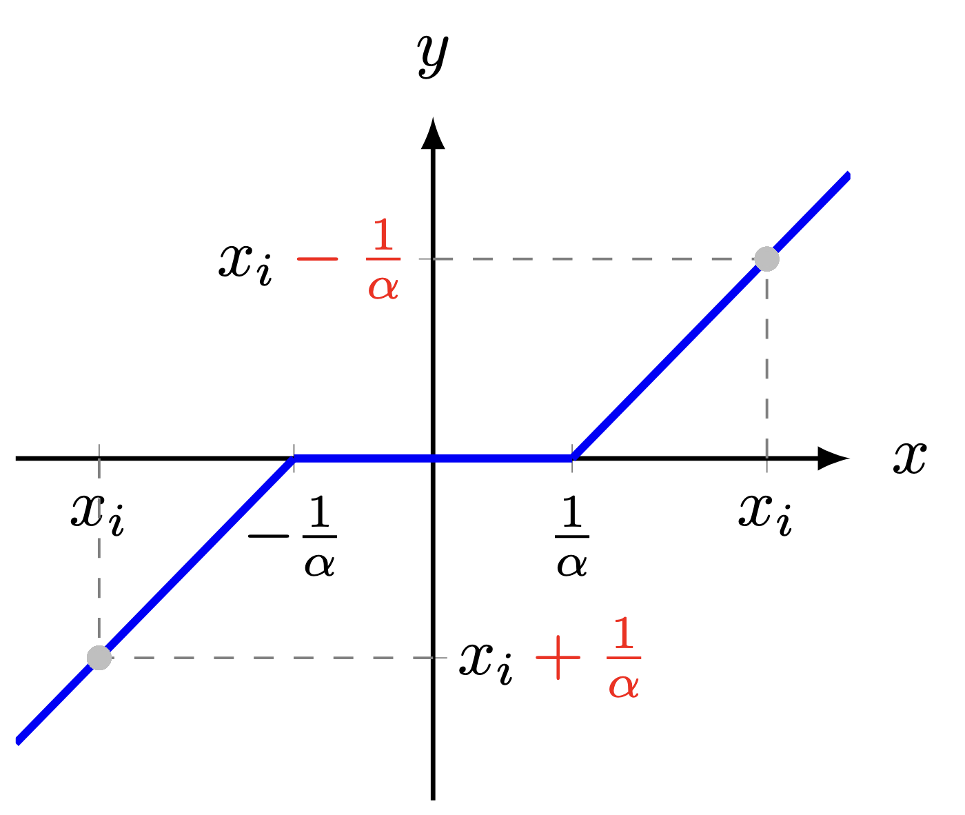
Figure 7. Illustration of the shrinkage operator for solving the $\ell_1$-norm minimization problem.
III-F. $\boldsymbol{z}$-Subproblem
In terms of the variable $\boldsymbol{z}$, the partial derivative of the augmented Lagrangian function with respect to $\mathcal{P}_{\Omega}(\boldsymbol{z})$ is given by
\[\begin{aligned} \frac{\partial\mathcal{L}_{\lambda}(\boldsymbol{x},\boldsymbol{z},\boldsymbol{w})}{\partial\mathcal{P}_{\Omega}(\boldsymbol{z})}=&\gamma\mathcal{P}_{\Omega}(\boldsymbol{z}-\boldsymbol{y})+\lambda\mathcal{P}_{\Omega}(\boldsymbol{z}-\boldsymbol{x})-\mathcal{P}_{\Omega}(\boldsymbol{w}) \\ =&(\gamma+\lambda)\mathcal{P}_{\Omega}(\boldsymbol{z})-\mathcal{P}_{\Omega}(\gamma\boldsymbol{y}+\lambda\boldsymbol{x}+\boldsymbol{w}) \end{aligned}\]while
\[\begin{aligned} \frac{\partial\mathcal{L}_{\lambda}(\boldsymbol{x},\boldsymbol{z},\boldsymbol{w})}{\partial\mathcal{P}_{\Omega}^{\perp}(\boldsymbol{z})}=&\lambda\mathcal{P}_{\Omega}^{\perp}(\boldsymbol{z}-\boldsymbol{x})-\mathcal{P}_{\Omega}^{\perp}(\boldsymbol{w}) \\ =&\lambda\mathcal{P}_{\Omega}^{\perp}(\boldsymbol{z})-\mathcal{P}_{\Omega}^{\perp}(\lambda\boldsymbol{x}+\boldsymbol{w}) \end{aligned}\]As a result, letting the partial derivative of the augmented Lagrangian function with respect to $\boldsymbol{z}$ be a zero vector, the least squares solution is given by
\[\begin{aligned} \boldsymbol{z}:=&\Bigl\{\boldsymbol{z}\mid \frac{\partial\mathcal{L}_{\lambda}(\boldsymbol{x},\boldsymbol{z},\boldsymbol{w})}{\partial\mathcal{P}_{\Omega}(\boldsymbol{z})}+\frac{\partial\mathcal{L}_{\lambda}(\boldsymbol{x},\boldsymbol{z},\boldsymbol{w})}{\partial\mathcal{P}_{\Omega}^{\perp}(\boldsymbol{z})}=\boldsymbol{0}\Bigr\} \\ =&\frac{1}{\gamma+\lambda}\mathcal{P}_{\Omega}(\gamma\boldsymbol{y}+\lambda\boldsymbol{x}+\boldsymbol{w})+\frac{1}{\lambda}\mathcal{P}_{\Omega}^{\perp}(\lambda\boldsymbol{x}+\boldsymbol{w}) \end{aligned}\]where the partial derivative of the augmented Lagrangian function with respect to the variable $\boldsymbol{z}$ is the combination of variables \(\mathcal{P}_{\Omega}(\boldsymbol{z})\) and \(\mathcal{P}_{\Omega}^\perp(\boldsymbol{z})\).
import numpy as np

def update_z(y_train, pos_train, x, w, lmbda, gamma):
    z = x + w / lmbda
    z[pos_train] = (gamma * y_train + lmbda * z[pos_train]) / (gamma + lmbda)
    return z
III-G. Time Series Imputation
As shown in Figure 8, we randomly remove 95% observations as missing values, and we only have 14 volume observations (i.e., 14 blue dots) for the reconstruction. The circulant matrix nuclear norm minimization can capture the global trends from partial observations.
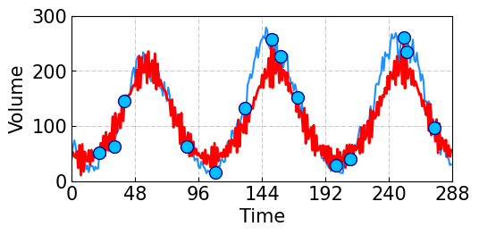
Figure 8. Univariate time series imputation on the freeway traffic volume time series. The blue and red curves correspond to the ground truth time series and reconstructed time series achieved by the circulant matrix nuclear norm minimization.
Please reproduce the experiments by following the Jupyter Notebook, which is available at the LCR repository on GitHub. For the supplementary material, please check out Appendix I(A).
IV. Laplacian Convolutional Representation
IV-A. Representing Circulant Graphs by Laplacian Kernels, Instead of Laplacian Matrices?
Laplacian convolutional representation model proposed by Chen et al., (2024) integrates local trends of time series into the global trend modeling via the use of circulant matrix nuclear norm minimization. As shown in Figure 1(b), the transition of time series data points can be naively modeled by smoothing regularization. We started by introducing Laplacian matrix to represent the prescribed relationship among time series data points.

Figure 9. Undirected and circulant graphs on the data points ${x_1,x_2,x_3,x_4,x_5}$ with certain degrees. The degrees of the left and right graphs are 2 and 4, respectively.
By definition, the Laplacian matrix of a circulant graph (see e.g., Figure 9) is a circulant matrix (refer to the formal definition of circulant matrix in Section II-C). In Figure 9, the Laplacian matrix corresponding to the left graph is expressed as
\[\boldsymbol{L}=\begin{bmatrix} 2 & -1 & 0 & 0 & -1 \\ -1 & 2 & -1 & 0 & 0 \\ 0 & -1 & 2 & -1 & 0 \\ 0 & 0 & -1 & 2 & -1 \\ -1 & 0 & 0 & -1 & 2 \end{bmatrix}=\mathcal{C}(\boldsymbol{\ell})\in\mathbb{R}^{5\times 5}\]while the Laplacian matrix for the right one is
\[\boldsymbol{L}=\begin{bmatrix} 4 & -1 & -1 & -1 & -1 \\ -1 & 4 & -1 & -1 & -1 \\ -1 & -1 & 4 & -1 & -1 \\ -1 & -1 & -1 & 4 & -1 \\ -1 & -1 & -1 & -1 & 4 \end{bmatrix}=\mathcal{C}(\boldsymbol{\ell})\in\mathbb{R}^{5\times 5}\]In both two Laplacian matrices, the diagonal entries are the degrees of circulant graphs. The vector $\boldsymbol{\ell}\in\mathbb{R}^{5}$ encodes the structural information of these graphs, capturing their underlying circulant structure. In this work, we define the first column of Laplacian matrices as the Laplacian kernels (Chen et al., 2024):
\[\boldsymbol{\ell}=(2,-1,0,0,-1)^\top\in\mathbb{R}^{5}\]and
\[\boldsymbol{\ell}=(4,-1,-1,-1,-1)^\top\in\mathbb{R}^{5}\]respectively.
Laplacian Kernel. Given any time series $\boldsymbol{x}\in\mathbb{R}^{T}$, suppose $\tau\in\mathbb{Z}^{+}$ be the kernel size of an undirected and circulant graph, then the Laplacian kernel is defined as
\[\color{gray}\boldsymbol{\ell}\triangleq(2\tau,\underbrace{-1,\cdots,-1}_{\tau},0,\cdots,0,\underbrace{-1,\cdots,-1}_{\tau})^\top\in\mathbb{R}^{T}\]which is the first column of the Laplacian matrix and the degree matrix is diagonalized with entries $2\tau$.
IV-B. Reformulating Temporal Regularization with Circular Convolution
In machine learning, one can write the temporal regularization on the time series $\boldsymbol{x}\in\mathbb{R}^{T}$, e.g.,
\[\mathcal{R}(\boldsymbol{x})=\frac{1}{2}\|\boldsymbol{L}\boldsymbol{x}\|_2^2\]Since the Laplacian matrix $\boldsymbol{L}$ is a circulant matrix, the matrix-vector multiplication $\boldsymbol{L}\boldsymbol{x}$ can be reformulated as a circular convolution between Laplacian kernel $\boldsymbol{\ell}$ and the vector $\boldsymbol{x}$, i.e., $\boldsymbol{\ell}\star\boldsymbol{x}$. For instance, given a Laplacian kernel $\boldsymbol{\ell}=(2,-1,0,0,-1)^{\top}$, we have
\[\boldsymbol{L}\boldsymbol{x}=\begin{bmatrix} 2 & -1 & 0 & 0 & -1 \\ -1 & 2 & -1 & 0 & 0 \\ 0 & -1 & 2 & -1 & 0 \\ 0 & 0 & -1 & 2 & -1 \\ -1 & 0 & 0 & -1 & 2 \\ \end{bmatrix} \begin{bmatrix} x_1 \\ x_2 \\ x_3 \\ x_4 \\ x_5 \end{bmatrix}=\begin{bmatrix} 2 \\ -1 \\ 0 \\ 0 \\ -1 \\ \end{bmatrix}\star\begin{bmatrix} x_1 \\ x_2 \\ x_3 \\ x_4 \\ x_5 \end{bmatrix}=\boldsymbol{\ell}\star\boldsymbol{x}\]As can be seen, this Laplacian kernel can build local correlations for the vector $\boldsymbol{x}$. Thus, the purpose of introducing Laplacian kernels on time series is local trend modeling with temporal regularization such that
\[\mathcal{R}(\boldsymbol{x})=\frac{1}{2}\|\boldsymbol{L}\boldsymbol{x}\|_2^2=\frac{1}{2}\|\boldsymbol{\ell}\star\boldsymbol{x}\|_2^2\]As a matter of fact, we have several motivations and reasons for reformulating temporal regularization with circular convolution. Among them, there are some important properties inspired us a lot. In particular, one of the most useful properties of circular convolution is its relationship with discrete Fourier transform, i.e.,
\[\mathcal{R}(\boldsymbol{x})=\frac{1}{2}\|\boldsymbol{\ell}\star\boldsymbol{x}\|_2^2=\frac{1}{2T}\|\mathcal{F}(\boldsymbol{\ell})\circ\mathcal{F}(\boldsymbol{x})\|_2^2 \tag{21}\]where $\mathcal{F}(\cdot)$ denotes the discrete Fourier transform. The symbol $\circ$ is the Hadamard product or element-wise product.
Example 10. Given vectors $\boldsymbol{x}=(0,1,2,3,4)^\top$ and $\boldsymbol{\ell}=(2,-1,0,0,-1)^\top$, the circular convolution is
\[\color{gray}\boldsymbol{\ell}\star\boldsymbol{x}=\mathcal{C}(\boldsymbol{\ell})\boldsymbol{x}=\begin{bmatrix} 2 & -1 & 0 & 0 & -1 \\ -1 & 2 & -1 & 0 & 0 \\ 0 & -1 & 2 & -1 & 0 \\ 0 & 0 & -1 & 2 & -1 \\ -1 & 0 & 0 & -1 & 2 \\ \end{bmatrix} \begin{bmatrix} 0 \\ 1 \\ 2 \\ 3 \\ 4 \\ \end{bmatrix} =\begin{bmatrix} -5 \\ 0 \\ 0 \\ 0 \\ 5 \end{bmatrix}\]and the regularization is
\[\color{gray}\mathcal{R}(\boldsymbol{x})=\frac{1}{2}\|\boldsymbol{\ell}\star\boldsymbol{x}\|_2^2=\frac{1}{2}((-5)^2+5^2)=25\]How to compute the regularization $\mathcal{R}(\boldsymbol{x})$ with fast Fourier transform? 1) Compute the fast Fourier transform on $\boldsymbol{\ell}$ and $\boldsymbol{x}$ as $\mathcal{F}(\boldsymbol{\ell})$ and $\mathcal{F}(\boldsymbol{x})$, respectively; 2) Compute the regularization as $\mathcal{R}(\boldsymbol{x})=25$.
import numpy as np

ell = np.array([0, 1, 2, 3, 4])
x = np.array([2, -1, 0, 0, -1])
f_ell = np.fft.fft(ell)
f_x = np.fft.fft(x)
print('Regularization R(x):')
print(np.linalg.norm(f_ell * f_x, 2) ** 2 / (2 * len(x)))
V. Learning Interpretable Convolutional Kernels
V-A. Convolutional Kernels
On the univariate time series $\boldsymbol{x}\in\mathbb{R}^{T}$ in the form of a vector, the circular convolution between time series $\boldsymbol{x}\in\mathbb{R}^{T}$ and convolutional kernel $\boldsymbol{\theta}\in\mathbb{R}^{T}$ can be constructed with certain purposes. The expression is formally defined by $\boldsymbol{x}\star\boldsymbol{\theta}\in\mathbb{R}^{T}$. When using this kernel to characterize the temporal correlations of time series, one simple yet interesting idea is making the loss of circular convolution, namely, $|\boldsymbol{x}\star\boldsymbol{\theta}|_2^2$, as small as possible. However, the optimization problem
\[\min_{\boldsymbol{\theta}}\,\|\boldsymbol{x}\star\boldsymbol{\theta}\|_2^2\]is ill-posed because the optimal solution is all entries of kernel $\boldsymbol{\theta}$ being zeros. To address this challenge, we assume that the first entry of $\boldsymbol{\theta}$ is one and the following $T-1$ entries are $-\boldsymbol{w}$ in which $\boldsymbol{w}\in\mathbb{R}^{T-1}$ is a non-negative vector. Thus, the optimization problem becomes
\[\begin{aligned} \min_{\boldsymbol{w}\geq 0}\,&\|\boldsymbol{x}\star\boldsymbol{\theta}\|_2^2 \\ \text{s.t.}\,&\boldsymbol{\theta}=\begin{bmatrix} 1 \\ -\boldsymbol{w} \end{bmatrix} \end{aligned} \tag{22}\]where the constraint is significant for minimizing the objective function.
V-B. Sparse Linear Regression
Recall that the circular convolution can be converted into a linear transformation with circulant matrix, namely, $\boldsymbol{\theta}\star\boldsymbol{x}=\mathcal{C}(\boldsymbol{\theta})\boldsymbol{x}$. If we let $\boldsymbol{\Theta}=\mathcal{C}(\boldsymbol{\theta})\in\mathbb{R}^{T\times T}$, then this matrix can be expressed as a matrix polynomial such that
\[\boldsymbol{\Theta}=\boldsymbol{I}_{T}-w_1\boldsymbol{F}-w_2\boldsymbol{F}^2-\cdots-w_{T-1}\boldsymbol{F}^{T-1} \tag{23}\]which is equivalent to
\[\boldsymbol{\theta}=(1,-w_1,-w_2,\cdots,-w_{T-1})^\top=\begin{bmatrix} 1 \\ -\boldsymbol{w} \end{bmatrix} \tag{24}\]where $\boldsymbol{I}_{T}\in\mathbb{R}^{T\times T}$ is the identity matrix and the time-shift matrix is given by
\[\boldsymbol{F}=\begin{bmatrix} 0 & 0 & 0 & \cdots & 0 & 1 \\ 1 & 0 & 0 & \cdots & 0 & 0 \\ 0 & 1 & 0 & \cdots & 0 & 0 \\ \vdots & \vdots & \vdots & \ddots & \vdots \\ 0 & 0 & 0 & \cdots & 0 & 0 \\ 0 & 0 & 0 & \cdots & 1 & 0 \\ \end{bmatrix}\in\mathbb{R}^{T\times T}\]Example 11. Any square matrix can be multiplied by itself and the result is a square matrix of the same size. Given a time-shift matrix of size $5\times 5$ such that
\[\color{gray}\boldsymbol{F}=\begin{bmatrix} 0 & 0 & 0 & 0 & 1 \\ 1 & 0 & 0 & 0 & 0 \\ 0 & 1 & 0 & 0 & 0 \\ 0 & 0 & 1 & 0 & 0 \\ 0 & 0 & 0 & 1 & 0 \end{bmatrix}\]Then, the power of matrix $\boldsymbol{F}$ can be written as follows,
\[\color{gray}\boldsymbol{F}^2=\begin{bmatrix} 0 & 0 & 0 & 0 & 1 \\ 1 & 0 & 0 & 0 & 0 \\ 0 & 1 & 0 & 0 & 0 \\ 0 & 0 & 1 & 0 & 0 \\ 0 & 0 & 0 & 1 & 0 \end{bmatrix}\begin{bmatrix} 0 & 0 & 0 & 0 & 1 \\ 1 & 0 & 0 & 0 & 0 \\ 0 & 1 & 0 & 0 & 0 \\ 0 & 0 & 1 & 0 & 0 \\ 0 & 0 & 0 & 1 & 0 \end{bmatrix}=\begin{bmatrix} 0 & 0 & 0 & 1 & 0 \\ 0 & 0 & 0 & 0 & 1 \\ 1 & 0 & 0 & 0 & 0 \\ 0 & 1 & 0 & 0 & 0 \\ 0 & 0 & 1 & 0 & 0 \end{bmatrix}\] \[\color{gray}\boldsymbol{F}^3=\begin{bmatrix} 0 & 0 & 0 & 1 & 0 \\ 0 & 0 & 0 & 0 & 1 \\ 1 & 0 & 0 & 0 & 0 \\ 0 & 1 & 0 & 0 & 0 \\ 0 & 0 & 1 & 0 & 0 \end{bmatrix}\begin{bmatrix} 0 & 0 & 0 & 0 & 1 \\ 1 & 0 & 0 & 0 & 0 \\ 0 & 1 & 0 & 0 & 0 \\ 0 & 0 & 1 & 0 & 0 \\ 0 & 0 & 0 & 1 & 0 \end{bmatrix}=\begin{bmatrix} 0 & 0 & 1 & 0 & 0 \\ 0 & 0 & 0 & 1 & 0 \\ 0 & 0 & 0 & 0 & 1 \\ 1 & 0 & 0 & 0 & 0 \\ 0 & 1 & 0 & 0 & 0 \end{bmatrix}\] \[\color{gray}\boldsymbol{F}^4=\begin{bmatrix} 0 & 0 & 1 & 0 & 0 \\ 0 & 0 & 0 & 1 & 0 \\ 0 & 0 & 0 & 0 & 1 \\ 1 & 0 & 0 & 0 & 0 \\ 0 & 1 & 0 & 0 & 0 \end{bmatrix}\begin{bmatrix} 0 & 0 & 0 & 0 & 1 \\ 1 & 0 & 0 & 0 & 0 \\ 0 & 1 & 0 & 0 & 0 \\ 0 & 0 & 1 & 0 & 0 \\ 0 & 0 & 0 & 1 & 0 \end{bmatrix}=\begin{bmatrix} 0 & 1 & 0 & 0 & 0 \\ 0 & 0 & 1 & 0 & 0 \\ 0 & 0 & 0 & 1 & 0 \\ 0 & 0 & 0 & 0 & 1 \\ 1 & 0 & 0 & 0 & 0 \end{bmatrix}\]As a result, the loss function constructed by circular convolution is
\[\|\boldsymbol{x}\star\boldsymbol{\theta}\|_2^2=\|\mathcal{C}(\boldsymbol{x})\boldsymbol{\theta}\|_2^2=\|\boldsymbol{x}-\boldsymbol{A}\boldsymbol{w}\|_2^2 \tag{25}\]where the auxiliary matrix $\boldsymbol{A}\in\mathbb{R}^{T\times (T-1)}$ is comprised of the last $T-1$ columns of the circulant matrix $\mathcal{C}(\boldsymbol{x})\in\mathbb{R}^{T\times T}$, namely,
\[\boldsymbol{A}=\begin{bmatrix} x_{T} & x_{T-1} & x_{T-2} & \cdots & x_{2} \\ x_{1} & x_{T} & x_{T-1} & \cdots & x_{3} \\ x_{2} & x_{1} & x_{T} & \cdots & x_{4} \\ \vdots & \vdots & \vdots & \ddots & \vdots \\ x_{T-2} & x_{T-3} & x_{T-4} & \cdots & x_{T} \\ x_{T-1} & x_{T-2} & x_{T-3} & \cdots & x_{1} \\ \end{bmatrix}\]where the matrix $\mathcal{C}(\boldsymbol{x})$ is separated into the vector $\boldsymbol{x}$ (i.e., first column of $\mathcal{C}(\boldsymbol{x})$) and the matrix $\boldsymbol{A}$ (i.e., last $T-1$ columns of $\mathcal{C}(\boldsymbol{x})$), see Figure 10 and Figure 11 for illustrations.
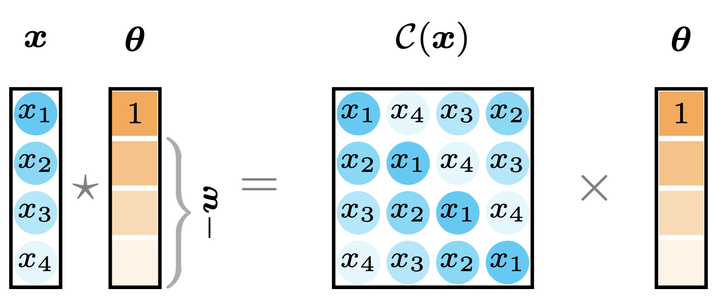
Figure 10. Illustration of circular convolution as the linear transformation with a circulant matrix.
As can be seen, one of the most intriguing properties is the circular convolution $\boldsymbol{x}\star\boldsymbol{\theta}$ can be converted into the expression $\boldsymbol{x}-\boldsymbol{A}\boldsymbol{w}$ (see Figure 11), which takes the form of a linear regression with the data pair ${\boldsymbol{x},\boldsymbol{A}}$.
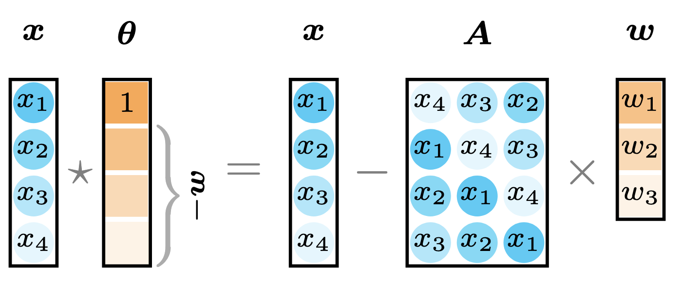
Figure 11. Illustration of circular convolution with a structured vector $\boldsymbol{\theta}$.
Example 12. Given vectors $\boldsymbol{x}=(0,1,2,3,4)^\top$ and $\boldsymbol{\theta}=(1,0,0,0,-1)^\top$, the circular matrix is
\[\color{gray}\mathcal{C}(\boldsymbol{x})=\begin{bmatrix} 0 & 4 & 3 & 2 & 1 \\ 1 & 0 & 4 & 3 & 2 \\ 2 & 1 & 0 & 4 & 3 \\ 3 & 2 & 1 & 0 & 4 \\ 4 & 3 & 2 & 1 & 0 \end{bmatrix}\]and the auxiliary matrix $\boldsymbol{A}$ is
\[\color{gray}\boldsymbol{A}=\begin{bmatrix} 4 & 3 & 2 & 1 \\ 0 & 4 & 3 & 2 \\ 1 & 0 & 4 & 3 \\ 2 & 1 & 0 & 4 \\ 3 & 2 & 1 & 0 \end{bmatrix}\]Thus, we can compute the circular convolution $\boldsymbol{x}\star\boldsymbol{\theta}$ by
\[\color{gray}\boldsymbol{x}-\boldsymbol{A}\boldsymbol{w}=\begin{bmatrix} 0 \\ 1 \\ 2 \\ 3 \\ 4 \\ \end{bmatrix}-\begin{bmatrix} 4 & 3 & 2 & 1 \\ 0 & 4 & 3 & 2 \\ 1 & 0 & 4 & 3 \\ 2 & 1 & 0 & 4 \\ 3 & 2 & 1 & 0 \end{bmatrix}\begin{bmatrix} 0 \\ 0 \\ 0 \\ 1 \\ \end{bmatrix}=\begin{bmatrix} 0 \\ 1 \\ 2 \\ 3 \\ 4 \\ \end{bmatrix}-\begin{bmatrix} 1 \\ 2 \\ 3 \\ 4 \\ 0 \\ \end{bmatrix}=\begin{bmatrix} -1 \\ -1 \\ -1 \\ -1 \\ 4 \end{bmatrix}\]V-C. Optimization Problem
To reinforce the model interpretability, we impose a sparsity constraint on the vector $\boldsymbol{w}$. This is extremely important for capturing local and nonlocal correlations of time series. The process of learning interpretable convolutional kernels can be formulated as follows,
\[\begin{aligned} \min_{\boldsymbol{w}\geq 0}\,&\|\boldsymbol{x}-\boldsymbol{A}\boldsymbol{w}\|_2^2 \\ \text{s.t.}\,&\|\boldsymbol{w}\|_0\leq \tau \end{aligned} \tag{26}\]where $\tau\in\mathbb{Z}^{+}$ is the sparsity level, i.e., the number of nonzero values.
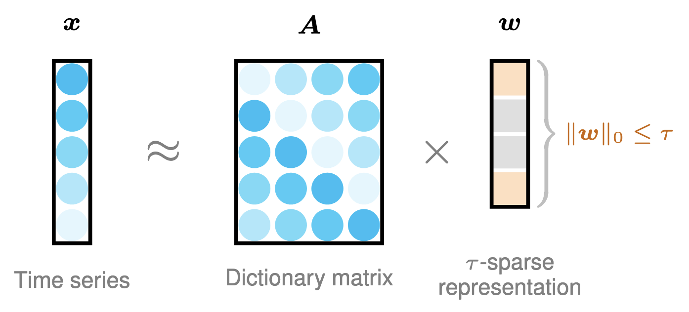
Figure 12. Illustration of learning $\tau$-sparse vector $\boldsymbol{w}$ from the time series $\boldsymbol{x}$ with the constructed formula as $\boldsymbol{x}\approx\boldsymbol{A}\boldsymbol{w}$.
$\ell_0$-Norm. For any vector $\boldsymbol{x}\in\mathbb{R}^{T}$, the $\ell_0$-norm is defined as follows,
\[\color{gray}\|\boldsymbol{x}\|_0=\operatorname{card}\{i\mid x_i\neq 0\}=|\operatorname{supp}(\boldsymbol{x})|\]where $\operatorname{card}{\cdot}$ and $\operatorname{supp}(\cdot)$ denote the cardinality and the support set of $\boldsymbol{x}$, respectively. For instance, given vector $\boldsymbol{x}=(0,1,2,3,4)^\top$, the support set is $\operatorname{supp}(\boldsymbol{x})={2,3,4,5}$ and the number of nonzero entries is $|\boldsymbol{x}|_0=4$.
V-D. Subspace Pursuit
Subspace Pursuit (SP), introduced by W. Dai and O. Milenkovic in 2008, is an iterative greedy algorithm used for sparse signal recovery, particularly in the context of compressed sensing. It aims to solve the $\ell_0$-norm minimization problem, which seeks to find the sparsest solution to an underdetermined system of linear equations. The $\ell_0$-norm counts the number of non-zero elements in a vector, making it a natural measure of sparsity. Generally speaking, one can use the subspace pursuit algorithm to solve the following optimization problem:
\[\begin{aligned} \min_{\boldsymbol{w}}\,&\|\boldsymbol{x}-\boldsymbol{A}\boldsymbol{w}\|_2^2 \\ \text{s.t.}\,&\|\boldsymbol{w}\|_0\leq \tau \end{aligned}\]
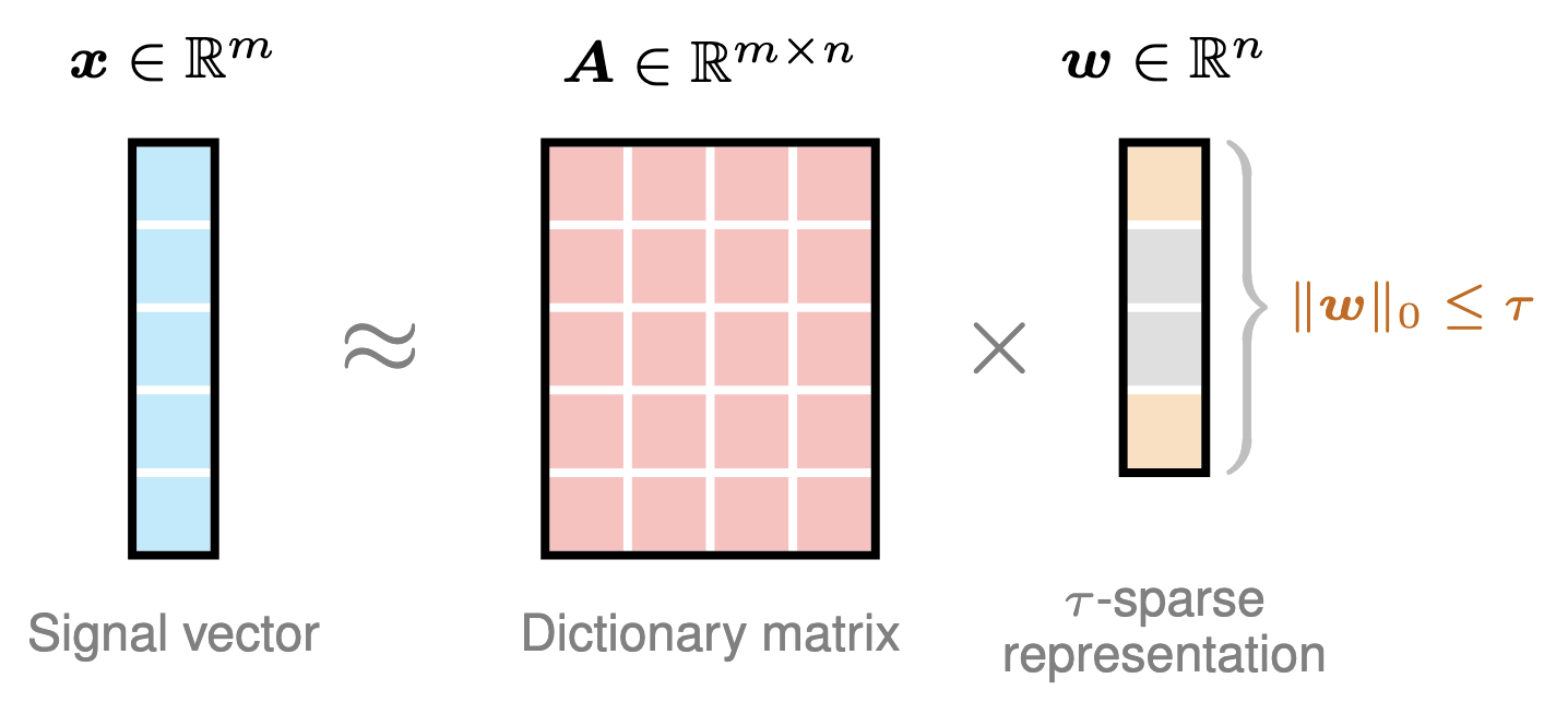
Figure 13. Illustration of learning $\tau$-sparse vector $\boldsymbol{w}$ from signal vector $\boldsymbol{x}$ and dictionary matrix $\boldsymbol{A}$ with the linear formula $\boldsymbol{x}\approx\boldsymbol{A}\boldsymbol{w}$.
Algorithm. Subspace Pursuit
- Input: Signal vector $\boldsymbol{x}\in\mathbb{R}^{m}$, dictionary matrix $\boldsymbol{A}\in\mathbb{R}^{m\times n}$, and sparsity level $\tau\in\mathbb{Z}^{+}$.
- Output: $\tau$-sparse vector $\boldsymbol{w}\in\mathbb{R}^{n}$ and index set $S$.
- Initialization: Sparse vector $\boldsymbol{w}=\boldsymbol{0}$ (i.e., zero vector), index set $S=\emptyset$ (i.e., empty set), and error vector $\boldsymbol{r}=\boldsymbol{x}$.
- while not stop do
- Find $\ell$ as the index set of the $\tau$ largest entries of $\lvert\boldsymbol{A}^\top\boldsymbol{r}\rvert$.
- $S:=S\cup\ell$.
- $\boldsymbol{w}_S:=\boldsymbol{A}_S^{\dagger}\boldsymbol{x}$ (least squares).
- Find $S$ as the index set of the $\tau$ largest entries of $\lvert\boldsymbol{w}\rvert$.
- $\boldsymbol{w}_S:=\boldsymbol{A}_S^{\dagger}\boldsymbol{x}$ (least squares again!).
- Set $w_i=0$ for all $i\notin S$.
- $\boldsymbol{r}=\boldsymbol{x}-\boldsymbol{A}_S\boldsymbol{w}_S$.
- end
By letting the objective function be $f$, then the derivative of $f$ is given by
\[\frac{\mathrm{d}\,f}{\mathrm{d}\,\boldsymbol{w}}=-\boldsymbol{A}^\top\underbrace{(\boldsymbol{x}-\boldsymbol{A}\boldsymbol{w})}_{\triangleq \boldsymbol{r}}\]Thus, the first step in the iterative process of subspace pursuit can select the $\tau$ largest absolute gradients (or absolute derivative values).
Acknowledgement. Thank you @Nina Cao for discussing the algorithmic implementation.
Example 13. Given vector $\boldsymbol{x}=(0,1,2,3,4)^\top$, the auxiliary matrix $\boldsymbol{A}$ (i.e., the last 4 columns of circulant matrix $\mathcal{C}(\boldsymbol{x})\in\mathbb{R}^{5\times 5}$) is
\[\color{gray}\boldsymbol{A}=\begin{bmatrix} 4 & 3 & 2 & 1 \\ 0 & 4 & 3 & 2 \\ 1 & 0 & 4 & 3 \\ 2 & 1 & 0 & 4 \\ 3 & 2 & 1 & 0 \end{bmatrix}\]The question is how to learn the vector $\boldsymbol{w}$ with sparsity level $\tau=2$ from the following optimization problem:
\[\color{gray}\begin{aligned} \min_{\boldsymbol{w}}\,&\|\boldsymbol{x}-\boldsymbol{A}\boldsymbol{w}\|_2^2 \\ \text{s.t.}\,&\|\boldsymbol{w}\|_0\leq \tau \end{aligned}\]In this case, the empirical solution of the decision variable is $\boldsymbol{w}=(0.44,0,0,0.44)^\top$. To reproduce it, the solution algorithm of subspace pursuit is given by
import numpy as np

def circ_mat(vec):
    n = vec.shape[0]
    mat = np.zeros((n, n))
    mat[:, 0] = vec
    for i in range(1, n):
        mat[:, i] = np.append(vec[-i :], vec[: n - i], axis = 0)
    return mat

def SP(x, tau, stop = np.infty, epsilon = 1e-2):
    t = x.shape[0]
    mat = circ_mat(x)
    A = mat[:, 1 :]
    r = x
    w = np.zeros(t - 1)
    S = np.array([])
    i = 0
    while np.linalg.norm(r, 2) > epsilon and i < stop:
        Ar = A.T @ r
        S0 = np.argsort(abs(Ar))[- tau :]
        S = np.append(S[:], S0[:]).astype(int)
        AS = A[:, S]
        w[S] = np.linalg.pinv(AS) @ x
        S = np.argsort(abs(w))[- tau :]
        w = np.zeros(t - 1)
        AS = A[:, S]
        w[S] = np.linalg.pinv(AS) @ x
        r = x - AS @ w[S]
        i += 1
        print('Indices of non-zero coefficients (support set):', S)
        print('Non-zero entries of sparse temporal kernel:', w[S])
        print()
    return w, S, r

x = np.array([0, 1, 2, 3, 4])
tau = 2 # sparsity level
w, S, r = SP(x, tau, 10)
V-F. Mixed-Integer Programming
There are often some special-purpose algorithms for solving constrained linear regression problems, see constrained least squares. Some examples of constraints include: 1) Non-negative least squares in which the vector $\boldsymbol{w}$ must satisfy the vector inequality $\boldsymbol{w}\geq 0$ (each entry must be either positive or zero); 2) Box-constrained least squares in which the vector $\boldsymbol{w}$ must satisfy the vector inequalities
\[\boldsymbol{b}_{\ell}\leq\boldsymbol{w}\leq \boldsymbol{b}_{u}\]In fact, the linear regression with sparsity constraints in the form of $\ell_0$-norm can be easily converted into a mixed-integer programming problem. Thus, the problem illustrated in Figure 12 is equivalent to
\[\begin{aligned} \min_{\boldsymbol{w},\boldsymbol{\beta}}\,&\|\boldsymbol{x}-\boldsymbol{A}\boldsymbol{w}\|_2^2 \\ \text{s.t.}\,&\begin{cases} \boldsymbol{\beta}\in\{0,1\}^{T-1} \\ 0\leq\boldsymbol{w}\leq\alpha\cdot\boldsymbol{\beta} \\ \displaystyle\sum_{t=1}^{T-1}\beta_t\leq \tau \end{cases} \end{aligned} \tag{27}\]where $\boldsymbol{\beta}\in\mathbb{R}^{T-1}$ is the binary decision variable. The weight $\alpha\in\mathbb{R}$ (possibly a great value for most cases) can control the upper bound of the vector $\boldsymbol{w}$. If $\beta_t=1$, then the value of $w_t$ is ranging between $0$ and $\alpha$. Otherwise, the value of $w_t$ is $0$ because both lower and upper bounds are $0$. In fact, the last constraint can also be written as follows,
\[\sum_{t=1}^{T-1}\beta_t =\|\boldsymbol{\beta}\|_1\leq \tau\]because the vector $\boldsymbol{\beta}$ is a non-negative vector.
Example 14. Given vector $\boldsymbol{x}=(0,1,2,3,4)^\top$, the auxiliary matrix $\boldsymbol{A}$ (i.e., the last 4 columns of circulant matrix $\mathcal{C}(\boldsymbol{x})\in\mathbb{R}^{5\times 5}$) is
\[\color{gray}\boldsymbol{A}=\begin{bmatrix} 4 & 3 & 2 & 1 \\ 0 & 4 & 3 & 2 \\ 1 & 0 & 4 & 3 \\ 2 & 1 & 0 & 4 \\ 3 & 2 & 1 & 0 \end{bmatrix}\]The question is how to learn the vector $\boldsymbol{w}$ with sparsity level $\tau=2$ from the following optimization problem:
\[\color{gray}\begin{aligned} \min_{\boldsymbol{w}\geq 0}\,&\|\boldsymbol{x}-\boldsymbol{A}\boldsymbol{w}\|_2^2 \\ \text{s.t.}\,&\|\boldsymbol{w}\|_0\leq \tau \end{aligned}\]In this case, the empirical solution of the decision variable is $\boldsymbol{w}=(0.44,0,0,0.44)^\top$. To reproduce it, the solution algorithm of mixed-integer programming is given by
import numpy as np
import cvxpy as cp

x = np.array([0, 1, 2, 3, 4])
A = circ_mat(x)[:, 1 :]
tau = 2 # sparsity level
d = A.shape[1]

# Variables
w = cp.Variable(d, nonneg=True)
beta = cp.Variable(d, boolean=True)

# Constraints
constraints = [cp.sum(beta) <= tau, w <= beta, w >= 0]

# Objective
objective = cp.Minimize(cp.sum_squares(x - A @ w))

# Problem
problem = cp.Problem(objective, constraints)
problem.solve(solver=cp.GUROBI)  # Ensure to use a solver that supports MIP

# Solution
print("Optimal beta:", w.value)
print("Active indices:", np.nonzero(beta.value > 0.5)[0])
Please install the optimization packages in-ahead, e.g., pip install gurobipy. One can also check out the optimization solvers in cvxpy:
import cvxpy as cp

print(cp.installed_solvers())
VI. Insight into Ridesharing Trip Time Series
The City of Chicago’s open data portal provides a large amount of human mobility data, including taxi trips and TNP ridesharing trips. Figure 14 shows the realistic time series data of ridesharing trips with a strong weekly periodicity, allowing one to examine the usage of interpretable convolutional kernels.
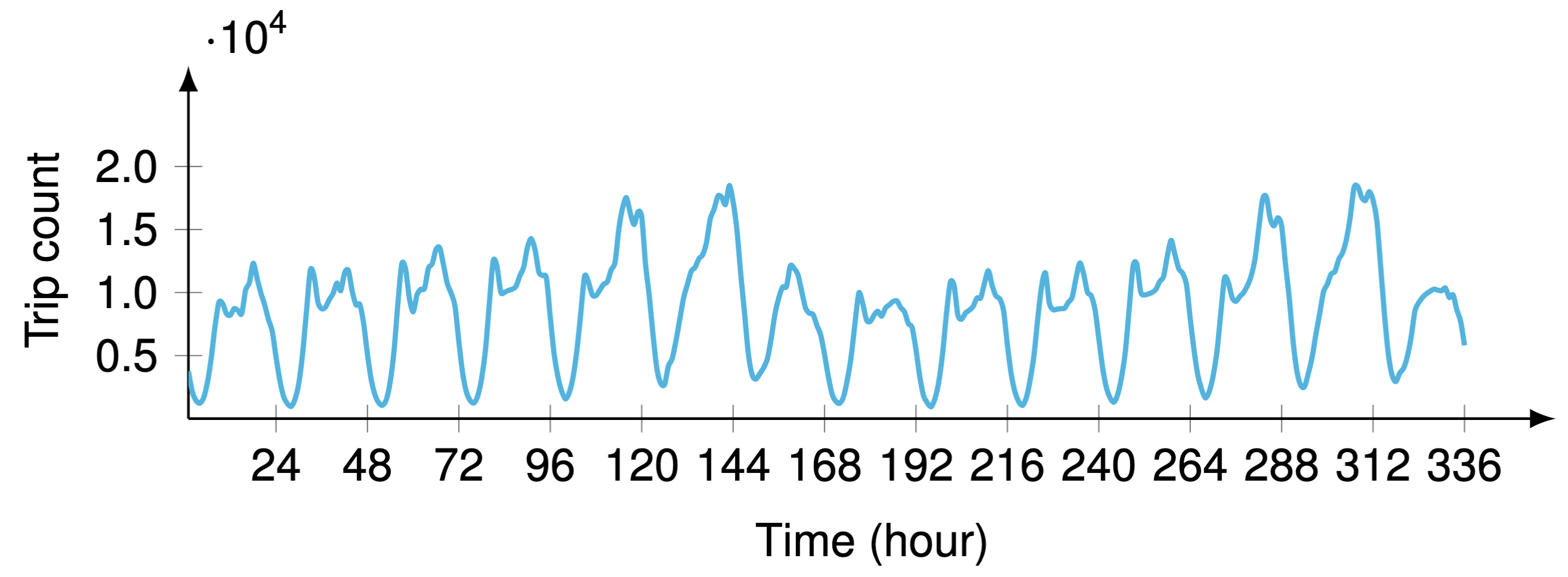
Figure 14. Hourly time series of aggregated ridesharing trip counts in the City of Chicago during the first two weeks (i.e., $2\times 7\times 24=336$ hours in total) since April 1, 2024. The time series exhibits weekly periodicity, referring to the regularity of human mobility.
Take the time series of Figure 14 as an example, the mixed-integer programming solver in CPLEX produces the temporal kernel $\boldsymbol{\theta}\triangleq (1,-\boldsymbol{w}^\top)^\top\in\mathbb{R}^{336}$ with
\[\boldsymbol{w}=(\underbrace{0.34}_{t=1},0,\cdots,0,\underbrace{0.33}_{t=168},0,\cdots,0,\underbrace{0.34}_{t=335})^\top\in\mathbb{R}^{335}\]where the sparsity level is set as $\tau=3$ in the constraint $|\boldsymbol{w}|_0\leq\tau$, or equivalently $|\boldsymbol{\beta}|_1\leq\tau$ on the binary decision variable $\boldsymbol{\beta}$. This result basically demonstrates local correlations such as $t=1$ and $335$, as well as the weekly seasonality at $t=168$. Below is the Python implementation of the mixed-integer programming solver with CPLEX.
import numpy as np
from docplex.mp.model import Model

def kernel_mip(data, tau):
    model = Model(name = 'Sparse Convolutional Kernel')
    T = data.shape[0]
    w = [model.continuous_var(lb = 0, name = f'w_{k}') for k in range(T - 1)]
    beta = [model.binary_var(name = f'beta_{k}') for k in range(T - 1)]
    error = [data[t] - model.sum(w[k] * data[t - k - 1] for k in range(T - 1)) for t in range(T)]
    model.minimize(model.sum(r ** 2 for r in error))
    model.add_constraint(model.sum(beta[k] for k in range(T - 1)) <= tau)
    for k in range(T - 1):
        model.add_constraint(w[k] <= beta[k])
    solution = model.solve()
    if solution:
        w_coef = np.array(solution.get_values(w))
        error = 0
        for t in range(T):
            a = data[t]
            for k in range(T - 1):
                a -= w_coef[k] * data[t - k - 1]
            error += a ** 2
        print('Objective function: {}'.format(error))
        ind = np.where(w_coef > 0)[0].tolist()
        print('Support set: ', ind)
        print('Coefficients w: ', w_coef[ind])
        print('Cardinality of support set: ', len(ind))
        return w_coef, ind
    else:
        print('No solution found.')
        return None

import numpy as np
import time

tensor = np.load('Chicago_rideshare_mob_tensor_24.npz')['arr_0'][:, :, : 14 * 24]
data = np.sum(np.sum(tensor, axis = 0), axis = 0)
tau = 3

start = time.time()
w, ind = kernel_mip(data, tau)
end = time.time()
print('Running time (s):', end - start)
For the entire implementation, please check out the Jupyter Notebook on GitHub. The processed time series dataset is available at the folder of Chicago-data.
VII. Quantifying Seasonality of Fluid Flow Data
Investigating fluid dynamic systems is of great interest for uncovering spatiotemporal coherent structures because dominant patterns exist in the flow field. To analyze the underlying seasonality of fluid dynamics, we aim to learn a sparse convolutional kernel on the cylinder wake dataset (i.e., fluid flow passing a circular cylinder) from the DMD book, see Figure 15 for some snapshots. The dataset is a multidimensional tensor of size $199\times 449\times 150$, representing $199$-by-$449$ vorticity fields with $150$ time snapshots.
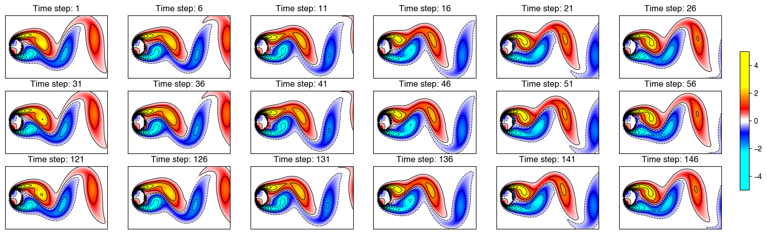
Figure 15. Matrix-variate time snapshots of the fluid flow dataset. This fluid flow dataset has the seasonality $\Delta t=30$. To demonstrate the periodic patterns, the time snapshots since $t=121$ are also presented.
As shown in Figure 15, these fluid flow snapshots are in the form of matrices
\[\boldsymbol{X}_{t}\in\mathbb{R}^{M\times N},\,t=1,2,\ldots,150\]with $M$ rows and $N$ columns, while the dataset is in the form of a tensor such that $\boldsymbol{\mathcal{X}}\in\mathbb{R}^{M\times N\times T}$ (element-wise, $x_{m,n,t}\in\mathbb{R}$). Thus, the optimization problem for learning sparse convolutional kernel can be formulated as follows,
\[\begin{aligned} \min_{\boldsymbol{w},\boldsymbol{\beta}}\,&\sum_{m=1}^{M}\sum_{n=1}^{N}\|\boldsymbol{x}_{m,n}-\boldsymbol{A}_{m,n}\boldsymbol{w}\|_2^2 \\ \text{s.t.}\,&\begin{cases} \boldsymbol{\beta}\in\{0,1\}^{T-1} \\ 0\leq\boldsymbol{w}\leq\alpha\cdot\boldsymbol{\beta} \\ \displaystyle\sum_{t=1}^{T-1}\beta_{t}\leq\tau \quad\quad\color{blue}\text{(sparsity)} \\ \displaystyle\sum_{t=1}^{T-1}w_{t}=1 \quad\quad\color{blue}\text{(normalization)} \end{cases} \end{aligned} \tag{28}\]where $\tau\in\mathbb{Z}^{+}$ is the upper bound of the number of nonzero entries in $\boldsymbol{w}$.
On the fluid flow dataset, the mixed-integer programming solver in CPLEX produces the temporal kernel $\boldsymbol{\theta}\triangleq (1,-\boldsymbol{w}^\top)^\top\in\mathbb{R}^{150}$ with
\[\boldsymbol{w}=(\underbrace{0.34}_{t=1},0,\cdots,0,\underbrace{0.16}_{t=30},0,\cdots,0,\underbrace{0.16}_{t=120},0,\cdots,0,\underbrace{0.34}_{t=149})^\top\in\mathbb{R}^{149}\]where the sparsity level is set as $\tau=4$. This result is consistent with the subspace pursuit algorithm. This result basically demonstrates the seasonality with $\Delta t=30$. Below is the Python implementation of the mixed-integer programming solver with CPLEX.
import numpy as np
from docplex.mp.model import Model

def circ_mat(vec):
    n = vec.shape[0]
    mat = np.zeros((n, n))
    mat[:, 0] = vec
    for i in range(1, n):
        mat[:, i] = np.append(vec[-i :], vec[: n - i], axis = 0)
    return mat

def data2para(tensor):
    M, N, T = tensor.shape
    C = np.zeros((T - 1, T - 1))
    D = np.zeros(T - 1)
    for m in range(M):
        for n in range(N):
            A = circ_mat(tensor[m, n, :])[:, 1 :]
            C += A.T @ A
            D += A.T @ tensor[m, n, :]
    return C, D

def kernel_mip(C, D, tau):
    model = Model(name = 'Sparse Convolutional Kernel')
    T_minus_1 = D.shape[0]
    T = T_minus_1 + 1
    w = [model.continuous_var(lb = 0, name = f'w_{k}') for k in range(T - 1)]
    beta = [model.binary_var(name = f'beta_{k}') for k in range(T - 1)]
    model.minimize(model.sum(w[k] * model.sum(w[t] * C[k, t] for t in range(T - 1))
                             - 2 * w[k] * D[k] for k in range(T - 1)))
    model.add_constraint(model.sum(beta[k] for k in range(T - 1)) <= tau)
    model.add_constraint(model.sum(w[k] for k in range(T - 1)) == 1)
    for k in range(T - 1):
        model.add_constraint(w[k] <= beta[k])
    solution = model.solve()
    if solution:
        print(solution.get_values(w))
        w_coef = np.array(solution.get_values(w))
        ind = np.where(w_coef > 0)[0].tolist()
        print('Support set: ', ind)
        print('Coefficients w: ', w_coef[ind])
        print('Cardinality of support set: ', len(ind))
        return w_coef, ind
    else:
        print('No solution found.')
        return None

import time

tensor = np.load('tensor.npz')['arr_0']
C, D = data2para(tensor[:, :, : 150])
tau = 4

start = time.time()
w, ind = kernel_mip(C, D, tau)
end = time.time()
print('Running time (s):', end - start)
VIII. Concluding Remarks
From a time series analysis perspective, our modeling ideas can guide future research by using the properties of circular convolution and connecting with various signals. Because circular convolution is a core component in many machine learning tasks, this post could provide an example for how to leverage the circular convolution, discrete Fourier transform, and linear regression. While we focused on the time series imputation and the convolutional kernel learning problems, we hope that our modeling ideas will inspire others in the fields of machine learning and optimization.
(Posted by Xinyu Chen on April 17, 2024)