Foundation of Optimization
I. Gradient Descent Methods
A. Gradient Descent
B. Steepest Gradient Descent
C. Conjugate Gradient Descent
D. Proximal Gradient Descent
The optimization problem of LASSO is
where is the regularization parameter that controls the sparsity of variable
. The objective function has two terms:
The derivative of , namely, gradient, is given by
To elaborate on the -norm, one great challenge is that the function
is not necessarily differentiable. Thus, the derivative is expressed in terms of a subgradient. Suppose a standard
-norm minimization problem with a penalty term:
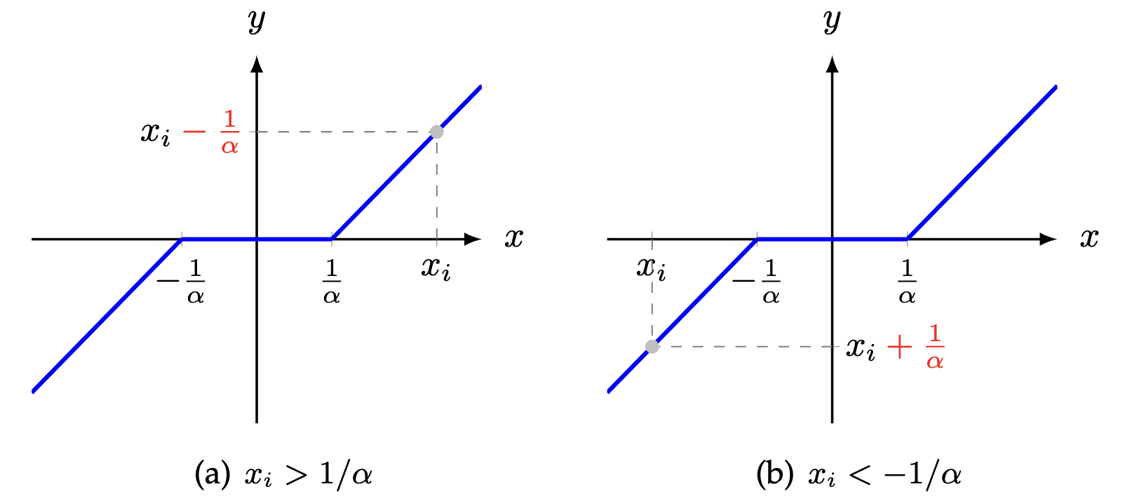
Figure 1. Illustration of the shrinkage operator for solving the -norm minimization problem.
II. Alternating Minimization
A. Alternating Least Squares
Alternating minimization is classical method for solving matrix and tensor factorization problems. In what follows, we use a matrix factorization example on the partially observed matrix to elaborate on the essential idea of alternating least squares. For any partially observed matrix with the observed index set
, the rank-
matrix factorization can be formulated on the partially observed entries of
, and it takes the following form:
where is a low rank for the approximation via the use of matrix factorization. In particular,
and
are factor matrices, while
is the weight parameter of the regularization terms for preventing overfitting. To represent the matrix factorization on the observed index set
of
,
denotes the orthogonal projection supported on
. For any
-th entry of
, the operator
can be described as follows,
Example 1. Given matrix , if the observed index set is
, then we have
Let the objective function of the aforementioned matrix factorization be (or
when mentioning all variables), then the partial derivatives of
with respect to
and
are given by
and
respectively. One can find the optimal solution to each subproblem by letting the partial derivative be zeros. In this case, the alternating minimization takes an iterative process by solving two subproblems:
The closed-form solution to each subproblem is given in the column vector of the factor matrix. If is the
-th column vector of the factor matrix
, then the least squares solution is
where is the
-th column vector of the factor matrix
. The least squares solution to
is
Since each subproblem in the alternating minimization scheme has least squares solutions, the scheme is also referred to as the alternating least squares.
Example 2.

Figure 1. Gaint panda with the gray scale. The image has pixels.
import matplotlib.pyplot as plt
from skimage import io

img = io.imread('gaint_panda_gray.jpg')
io.imshow(img)
plt.axis('off')
plt.show()
B. Alternating Minimization with Conjugate Gradient Descent
Smoothing matrix factorization on Panda
III. Alternating Direction Method of Multipliers
The Alternating Direction Method of Multipliers (ADMM) is an optimization algorithm designed to solve complex problems by decomposing them into a sequence of easy-to-solve subproblems (Boyd et al., 2011). ADMM efficiently handles both the primal and dual aspects of the optimization problem, ensuring convergence to a solution that satisfies the original problem’s constraints. The method synthesizes concepts from dual decomposition and augmented Lagrangian methods: dual decomposition divides the original problem into two or more subproblems, while the augmented Lagrangian methods use an augmented Lagrangian function to effectively handle constraints within the optimization process. This combination makes ADMM particularly powerful for solving large-scale and constrained optimization problems.
A. Problem Formulation
Typically, ADMM solves a class of optimization problems of the form
where and
are the optimization variables. The objective function has two convex functions
and
. In the constraint,
and
are matrices, while
is a vector.
B. Augmented Lagrangian Method
Augmented Lagrangian methods are usually used to solve constrained optimization problems, in which the algorithms replace a constrained optimization problem by a series of unconstrained problems and add penalty terms to the objective function. For the aforementioned constrained problem, the augmented Lagrangian method has the following unconstrained objective function:
where the dual variable is an estimate of the Lagrange multiplier, and
is a penalty parameter that controls the convergence rate. Notably, it is not necessary to take
as great as possible in order to solve the original constrained problem. The presence of dual variable
allows
to stay much smaller.
Thus, ADMM solves the original constrained problem by iteratively updating the variables ,
, and the dual variable
as follows,
In this case, ADMM performs between these updates util convergence. In terms of the variable , it takes the following subproblem:
In terms of the variable , we can write the subproblem as follows,
C. LASSO
Least Absolute Shrinkage and Selection Operator (LASSO) has wide applications to machine learning. The optimization problem of LASSO is
where is the regularization parameter that controls the sparsity of variable
. Using the variable splitting, this original problem can be rewritten to an optimization with a constraint:
First of all, the augmented Lagrangian function can be written as follows,
Thus, the variables ,
, and the dual variable
can be updated iteratively as follows,
In terms of the variable , the subproblem has a least squares solution:
where the partial derivative of the augmented Lagrangian function with respect to is given by
Let this partial derivative be a zero vector, then the closed-form solution is the least squares.
In terms of the variable , the subproblem is indeed an
-norm minimization:
Example 1.