Utilizing International Import and Export Trade Data from WTO Stats
The WTO Stats data portal contains statistical indicators related to WTO issues. Available time series cover merchandise trade and trade in services statistics (annual, quarterly and monthly), market access indicators (bound, applied & preferential tariffs), non-tariff information as well as other indicators. In this post, we consider the merchandise trade values, including annual, quarterly, and monthly import/export trade data in which the aunnual data has 18 product/sector types.
Content:
- Downloading annual data from the WTO Stats and preprocessing these data in Python (e.g.,
pandasandnumpy). - Visualizing international import and export trade values with
geopandas. - Representing the international import and export trade values as time series.
- Introducing tensor structure for representing the trade (quantity) data with (economy, product, year) dimensions.
WTO Stats Data
Data Preparation
The WTO Stats provides an open database, please check out https://stats.wto.org. For the purpose of analyzing international import/export trade, one should first consider select the following items in the download page:
Indicators->International trade statistics->Merchandise trade values(select all 6 items)Products/Sectors: 3 main types (i.e., agricultural products, fuels and mining products, manufactures) and 17 detailed typesYears(select from 2000 to 2022)
Then, one should apply the selection options and download the .csv data file. In this post, we make the import/export trade value data available at this GitHub repository.
In addition, to visualize results, one can download the countries’ shapefiles and boundaries at wri/wri-bounds on GitHub (or see this GitHub repository, including .shp).
Total Mechandise Trade Values (Annual)
In the dataset, one can use the pandas package to process the raw data. There are some steps to follow:
- Open the data with
pd.read_csv()(setsepandencoding) - Replace the column name
Reporting Economy ISO3A Codebyiso_a3, making it consistent with the.shpfile - Remove the
nanvalues in the columniso_a3 - Select
Total merchandise(the total trades over all product/sector types) - Create a 215-by-23 trade matrix with the
numpypackage, including trade values of 215 countires/regions over the past 23 years from 2000 to 2022
import pandas as pd
import numpy as np

data = pd.read_csv('WtoData.csv', sep = ',', encoding = 'latin-1')
data.rename(columns = {"Reporting Economy ISO3A Code": "iso_a3"}, inplace = True)
data = data[data['iso_a3'].notna()]
data = data.drop(data[data['iso_a3'] == 'EEC'].index) # Remove EEC
data = data[data['Indicator'] == 'Merchandise imports by product group \x96 annual']
data = data[data['Product/Sector'] == 'Total merchandise']

df = data.groupby('iso_a3').sum('Value').reset_index()
df = df.drop(['Year'], axis = 1)

year = 23
mat = np.zeros((df.shape[0], year))
for n in range(df.shape[0]):
    for t in range(year):
        mat[n, t] = data[(data['iso_a3'] == df['iso_a3'][n])
                          & (data['Year'] == 2000 + t)].Value.values.sum()

## Check out the trade values of each country/region
# data[data['iso_a3'] == df['iso_a3'][n]].sort_values(by = 'Year')
Next, we connect the trade values with the shapefile for visualization. Figure 1 shows the total merchandise trade values of imports reported by 215 countries/regions over the past 23 years from 2000 to 2022.
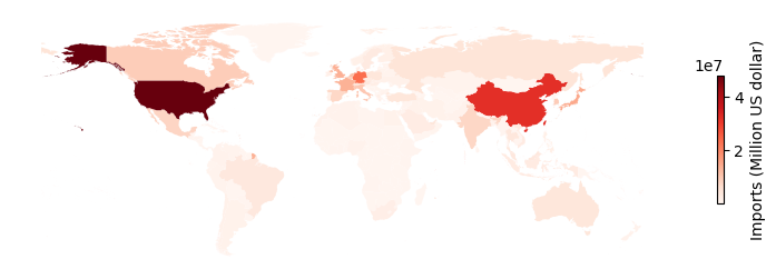
Figure 1. The total merchandise trade values of imports from 2000 to 2022.
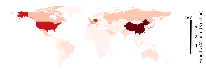
Figure 2. The total merchandise trade values of exports from 2000 to 2022.
For reproducing Figure 1, please check out the following codes.
import geopandas as gpd
import matplotlib.pyplot as plt

df['Value'] = np.sum(mat, axis = 1)
shape = gpd.read_file("cn_countries.shp")
trade = shape.set_index('iso_a3').join(df.set_index('iso_a3')).reset_index()

fig = plt.figure(figsize = (10, 3))
ax = fig.subplots(1)
trade.plot('Value', cmap = 'Reds', legend = True,
           legend_kwds = {'shrink': 0.5,
                          'label': 'Imports (Million US dollar)'}, ax = ax)
plt.xticks([])
plt.yticks([])
for _, spine in ax.spines.items():
    spine.set_visible(False)
plt.show()
fig.savefig("global_imports.png", bbox_inches = "tight")
International Trade Time Series
In the dataset, we hope to analyze the total mechandise trade values changing over time. Figure 3 shows the whole trend of the international trades from 2000 to 2022, experiencing three periods with significant trade reduction, e.g., 2008-2009, 2014-2016, and 2019-2020. Figure 4-6 present the total merchandise trades of the USA and China, respectively. Note that these figures can be reproduced by following these codes.

Figure 3. The total merchandise trade time series of imports from 2000 to 2022.

Figure 4. The total merchandise trade time series of USA imports from 2000 to 2022.

Figure 5. The total merchandise trade percentage (in the global trade) time series of USA imports from 2000 to 2022.
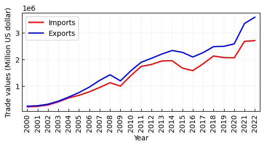
Figure 6. The total merchandise trade time series of China imports from 2000 to 2022.

Figure 7. The total merchandise trade percentage (in the global trade) time series of China imports from 2000 to 2022.
Trade Tensor
For the annual trade data, one additional dimension is the product/sector type. Despite the total merchandise, we have 17 product types listed as follows,
- Agricultural products
- Food
- Fuels and mining products
- Fuels
- Manufactures
- Iron and steel
- Chemicals
- Pharmaceuticals
- Machinery and transport equipment
- Office and telecom equipment
- Electronic data processing and office equipment
- Telecommunications equipment
- Integrated circuits and electronic components
- Transport equipment
- Automotive products
- Office and telecom equipment
- Textiles
- Clothing
One can create a tensor for representing trade values of 215 countries/regions, 17 products, and 23 years (i.e., from 2000 to 2022).
import pandas as pd
import numpy as np

data = pd.read_csv('WtoData.csv', sep = ',', encoding = 'latin-1')
data.rename(columns = {'Reporting Economy ISO3A Code': 'iso_a3'}, inplace = True)
data = data[data['iso_a3'].notna()]
data = data.drop(data[data['iso_a3'] == 'EEC'].index)
data = data[data['Indicator'] == 'Merchandise imports by product group \x96 annual']

prod = np.array(['Agricultural products', 'Food', 'Fuels and mining products',
                 'Fuels', 'Manufactures', 'Iron and steel', 'Chemicals',
                 'Pharmaceuticals', 'Machinery and transport equipment',
                 'Office and telecom equipment',
                 'Electronic data processing and office equipment',
                 'Telecommunications equipment',
                 'Integrated circuits and electronic components',
                 'Transport equipment', 'Automotive products',
                 'Textiles', 'Clothing'])
df = data.groupby('iso_a3').sum('Value').reset_index()
df = df.drop(['Year'], axis = 1)

year = 23
tensor = np.zeros((df.shape[0], prod.shape[0], year))
for n in range(df.shape[0]):
    for p in range(prod.shape[0]):
        for t in range(year):
            tensor[n, p, t] = data[(data['iso_a3'] == df['iso_a3'][n])
                                    & (data['Product/Sector'] == prod[p])
                                    & (data['Year'] == 2000 + t)].Value.values.sum()
np.savez_compressed('import_tensor.npz', tensor)
As one has such tensor (e.g., import_tensor.npz as a compressed array), it is possible to identify the spatial modes and product modes.
Big Trade Data
import pandas as pd

df = pd.read_csv("trade_i_baci_a_92.tsv.bz2", compression="bz2", sep='\t',
                 chunksize=1e+6)
data = df.get_chunk(1e+6)
data
import pandas as pd

data = pd.DataFrame(columns = ['exporter_id', 'importer_id', 'hs_code', 'year', 'value', 'quantity'])
chunksize = 10 ** 8
for chunk in pd.read_csv("trade_i_baci_a_92.tsv.bz2", compression = "bz2",
                         sep = '\t', chunksize = chunksize):
    df = pd.DataFrame()
    df['exporter_id'] = chunk['exporter_id'] # Exporter
    df['importer_id'] = chunk['importer_id'] # Importer
    df['hs_code'] = chunk['hs_code'] # Product
    df['year'] = chunk['year'] # Year
    df['value'] = chunk['value'] # Trade value
    df['quantity'] = chunk['quantity'] # Trade value
    data = pd.concat([data, df], ignore_index = True)
    del df
Here is a more detailed list of six-digit HS codes associated with AI and high-tech products in the dataset:
- Semiconductors and Electronic Components
- 854110: Diodes, other than photosensitive or light-emitting diodes.
- 854121: Transistors, other than photosensitive transistors, with a dissipation rate of less than 1 W.
- 854129: Other transistors.
- 854140: Photosensitive semiconductor devices, including photovoltaic cells, whether or not assembled in modules or made up into panels; light-emitting diodes.
- Instrumentation and Measuring Devices
- 903031: Multimeters without a recording device.
- 903039: Other instruments for measuring or checking voltage, current, resistance, or power, without a recording device.
- 903040: Instruments and apparatus, specially designed for telecommunications (for example, cross-talk meters, gain measuring instruments, distortion factor meters, psophometers).
- Robotics and Automation
- 842890: Other lifting, handling, loading, or unloading machinery.
- High-Tech Medical Equipment
- 901819: Other electro-diagnostic apparatus (including apparatus for functional exploratory examination or for checking physiological parameters).
- Optical and Photographic Instruments
- 900110: Optical fibers, optical fiber bundles and cables.
- 900120: Sheets and plates made of polarizing material.
- 900190: Lenses, prisms, mirrors, and other optical elements, of any material, unmounted, other than such elements of glass not optically worked.
- High-Tech Laboratory Equipment
- 902710: Gas or smoke analysis apparatus.
- 902720: Chromatographs and electrophoresis instruments.
- 902730: Spectrometers, spectrophotometers, and spectrographs using optical radiations (UV, visible, IR).
- 902750: Other instruments and apparatus using optical radiations (UV, visible, IR).
- Printed Circuit Boards
- 853400: Printed circuits.
- Sensors and Actuators
- 902610: Instruments and apparatus for measuring or checking the flow or level of liquids.
- 902620: Instruments and apparatus for measuring or checking pressure.
- Microelectromechanical Systems (MEMS)
- 901310: Telescopic sights for fitting to arms; periscopes; telescopes designed to form parts of machines, appliances, instruments, or apparatus of this chapter or Section XVI.
- 901380: Other optical devices, appliances, and instruments.
(Posted by Xinyu Chen on April 6, 2024.)